The Evolution of Solubility Prediction Methods
by Jonathon Vandezande · Feb 25, 2025
Solubility is one of the first concepts introduced in chemistry classes, yet its apparent simplicity belies its profound importance. Solubility governs how solutes interact with solvents; a principle that is critical for a long list of things, including:
- Modulating reaction rates
- Controlling drug crystallization
- Optimizing HPLC solvent systems
- Finding substitutes for hazardous solvents
- Controlling diffusion and minimizing stress cracking in polymers
There are several methods to tackle this challenge. These include traditional solubility parameter theories and, more recently, data-driven machine learning (ML) approaches. Traditional models, such as Hansen and Hildebrand solubility parameters, derive a small number of empirical parameters to determine the similarity of solute and solvent. Data-driven machine-learning methods have gained traction more recently, offering new ways to capture complex solute-solvent interactions.
Traditional Solubility Methods
Traditional solubility methods for solubility prediction work by measuring parameters for the solute and solvent. Following the common adage of "like dissolves like," molecules/polymers with similar values for the solubility parameters are likely to be soluble, while those with differing values are insoluble.
Hildebrand Solubility Parameter
Hildebrand solubility prediction uses a single parameter model (δ) wherein molecules with similar values of δ will likely be miscible. δ is derived from the energy needed to vaporize the molecule (cohesive energy density), and thus can easily be derived for many molecules. It is calculated as:
- – enthalpy of vaporization
- – molar volume
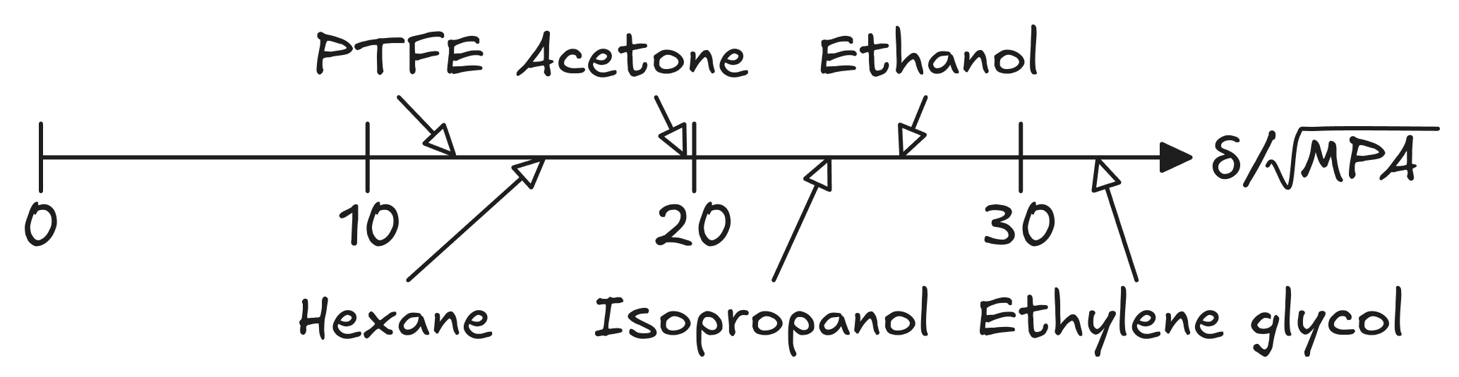
Figure 1: Hildebrand solubility parameters for common molecules.
Hildebrand solubility prediction can be useful for non-polar and slightly-polar molecules and polymers. However, it cannot account for deviations from Raoult's law due hydrogen-bonding or dipolar interactions, such as in ethanol or acetone, as solubility inherently cannot be described by a single number.
Hansen Solubility Parameters (HSP)
Hansen solubility parameters (HSP) attempt to correct the single parameter Hildebrand model by partitioning the solubility into dispersion (), dipolar interaction (), and hydrogen bonding () components. Each solute also has a solubility radius (), where solutes with a larger are soluble in a greater range of solvents. Each of these parameters is carefully measured and reported in . (If you think this unit is confusing, you're not alone! Why is hydrogen bonding being reported as the square root of pressure?)
Each molecule is assigned its own set of parameters (, , ), and a "Hansen sphere" of radius is plotted around the point (the sphere is scaled down by a factor of 2 in ). Solvents inside this sphere are likely to dissolve the molecule, and solvents outside of it are likely unable to dissolve it. Parameters for molecules/polymers that have yet to be measured can be estimated by a series of solubility experiments to triangulate the values.
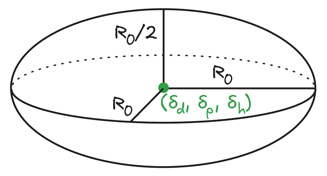
Figure 2: Hansen sphere showing the extent of solvents that can dissolve a molecule. The "sphere" is scaled by a factor of 2 in the dimension of , as differences in dispersion have a greater effect on solubility.
While only a limited number of solvents may solvate a given molecule, HSP can predict mixtures of miscible solvents that can together dissolve the molecule. The HSP of a mixture is just the mean of the parameters, weighted by the volume fraction of each component.
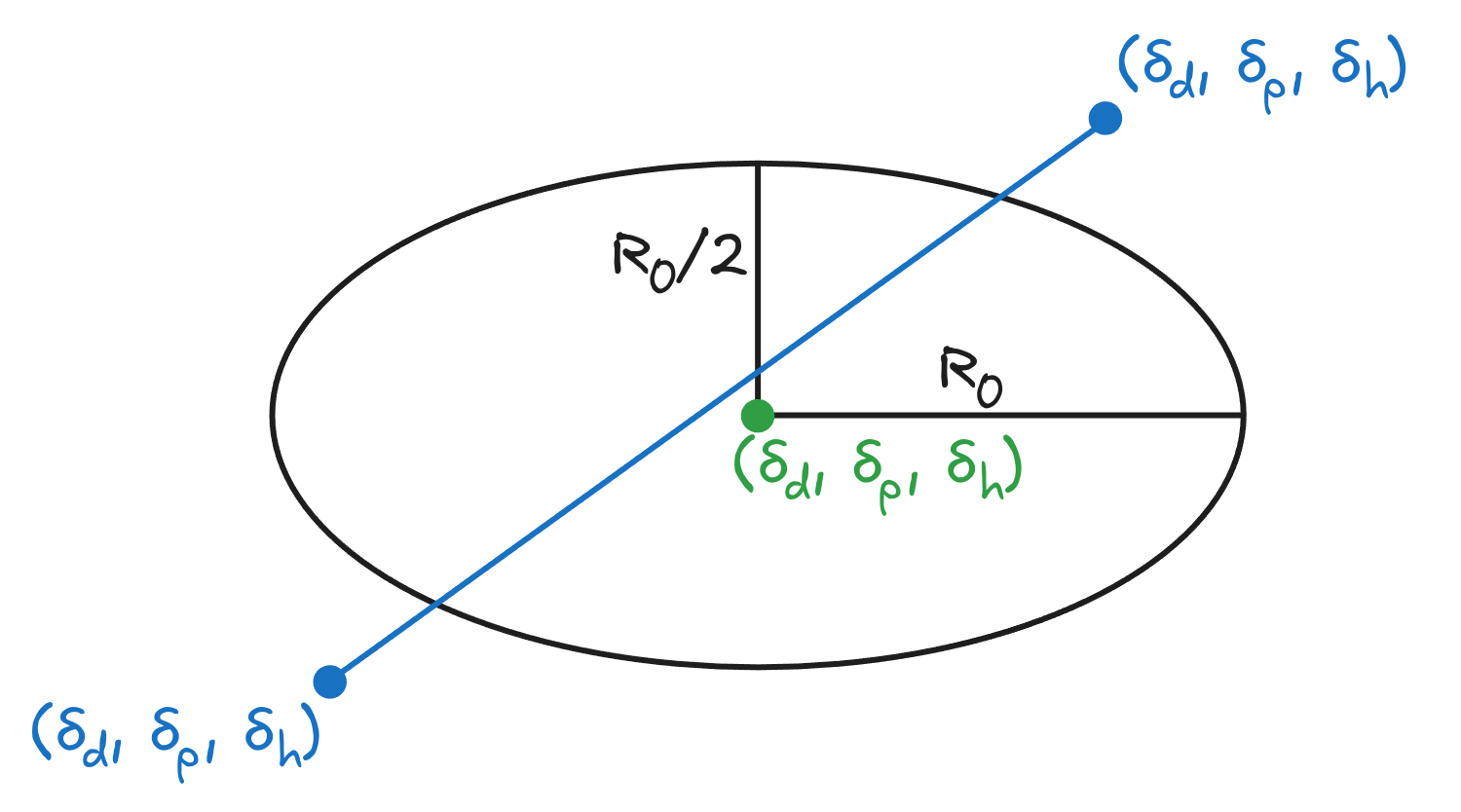
Figure 3: A mixture of solvents can solvate a molecule that is not miscible in either of the solvents individually. The optimal mixture can be found by drawing a line connecting the solvents and finding the nearest point to the solute. (Note: third dimension is removed for clarity.)
Hansen solubility parameters are particularly popular in polymer chemistry, where numerous measurements have been made of common solvents and polymers. They are often used to predict:
- Diffusion of solvents into polymers leading to swelling and stress-cracking
- Dispersion of inks, pigments, and carbon nanotubes
- Adhesion of paints and coatings to surfaces
- Miscibility of polymer blend
Extensions of Hansen solubility parameters have been made that include additional parameters and explicit temperature dependence, including the MOSCED 6-parameter model. However, these models require significantly more individual measurements. Attempts have been made to derive these parameters via computational modeling via MD, but it doing so can be expensive and it has not achieved widespread adoption.
Additionally, like most solubility models, HSP struggles with very small molecules that have strong hydrogen bonds, such as water and methanol. Water has a very strong hydrogen‐bonding parameter ( around 42 ), causing it to be very far from most organic molecules. However, it is actually an excellent solvent for many substances due to its ability to both donate and receive hydrogen bonds. Meanwhile, methanol's tendency to self-associate effectively hides some of its hydrogen‐bonding character and alters its measured and values. Modified values are often used to account for this behavior ((, , ) = (14.7, 5, 10) instead of the standard (14.5, 12.3, 22.3), but the accumulation of corrections can move the models away from its theoretical roots.
Machine-Learned Methods
The large number of corrections that are needed to precisely fit traditional solvation models can become rather unwieldy and makes addition of each new solvent time-consuming. Machine learning models forgo the exact semi-physical parameters and instead fit a model to a large amount of data. While these models often lose the explainability provided by traditional methods like HSP, they allow more accurate prediction of the actual solubility (as opposed to just the categorical soluble vs insoluble), straightforward prediction of temperature effects, and simple extension to previously unparameterized molecules.
Most ML methods start by engineering features from the target molecules. This can include fingerprinting (converting the functional groups of a molecule into a simple vector), explicitly calculating properties of a molecule (e.g. pKa, conformational flexibility, and aromaticity), or using the electron density (e.g. COSMOtherm/COSMO-RS). These features are then input into the model, which outputs a prediction for the solubility. Models can also be trained to output an uncertainty estimation for their results.
Thanks to feature engineering, it is possible to predict solubilities for previously unseen solutes and solvents, as long as molecules with similar properties were used in training the model. For example, if the model were trained on data containing n-pentane, n-hexane, and 1-aminopentane, it will likely perform well for 1-aminohexane, despite never having seen it.
Fastsolv
The fastsolv model from Lucas Attia, Jackson Burns, et al. is a deep-learning model that predicts solubility across a wide range of temperatures and a variety of organic solvents. It uses a data-driven approach, training on the large experimental solubility dataset BigSolDB, which contains 54,273 solubility measurements, 830 molecules, and 138 solvents. It leverages the fastprop library and mordred descriptors to engineer features for both the solute and the solvent, which, along with the temperature, are then passed into a neural network that predicts .
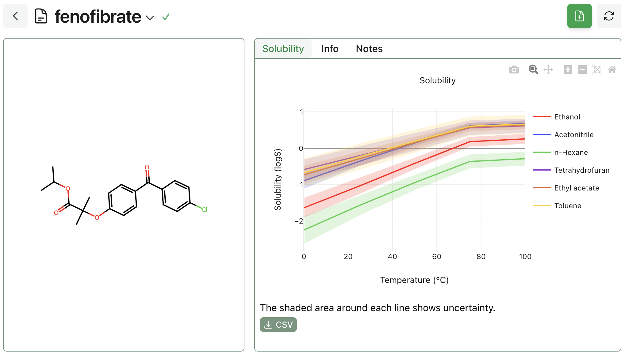
While HSP and many other empirical models merely classify whether a molecule is likely to soluble in a solvent, fastsolv can predict the actual solubility along with non-linear temperature effects and report the uncertainty in its predictions. Many experimental hours are devoted to determining the solubility curves of drug-like molecules, such as this paper on fenofibrate by Watterson et al., while fastolv can quickly provide such predictions across a variety of molecules and temperatures in less than a minute.
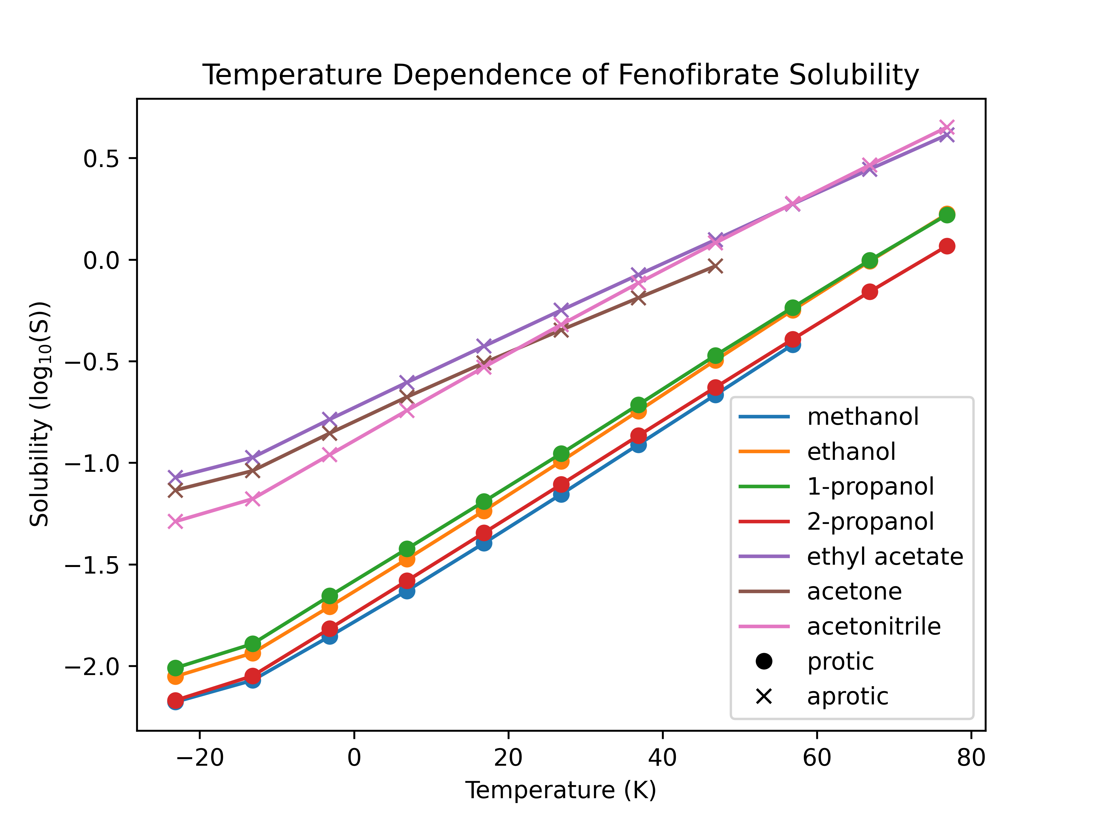
Figure 4: fastsolv predicted solubility of fenofibrate in common solvents showing increased solubility in aprotic solvents.
As seen in the experimental results, fenofibrate shows significantly higher solubility in polar aprotic solvents than in polar protic solvents, and a greater temperature dependence in acetonitrile than other aprotic solvents.
Solubility Prediction on Rowan
You can now run fastsolv solubility predictions on the Rowan platform. Rowan's solubility prediction tool built around fastsolv includes the following features.
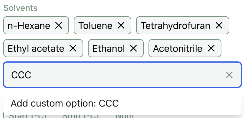
Default and Custom Solvents
A default set of commonly used non-polar, polar aprotic, and polar protic solvents is pre-populated on Rowan's solvation GUI. This GUI also supports arbitrary solvent selection, making it easy to predict solubility in whatever solvents you care about.
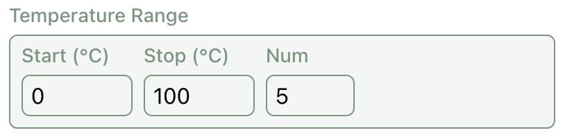
Temperature Selection
To predict the temperature dependence of solubility, Rowan's solubility predictor automatically predicts solubility across a range of temperatures. On the GUI, you can select the start point and end point of the range as well as a number points to sample along.
Responsive Graphs of Temperature-Dependent Solubility
The results of Rowan's solubility prediction are displayed on our GUI using Plotly.js, a powerful and responsive client-side graphing library. You can view the uncertainty of each prediction, show or hide solvents by clicking on the legend, and download a PNG of the graph to share or reference later.
API Access
For high-throughput computational needs or library-scale screening, Rowan provides access to the fastsolv model through our Python API.
To try Rowan's solubility prediction tool built around fastsolv, you can make a free account on our web-based computational platform. If you are interested in other solubility models or solubility-related features, we'd love to hear from you! You can reach us at contact@rowansci.com—we'd be happy to help you find the best solubility prediction method for your work.