Machine-Learning Methods for pH-Dependent Aqueous-Solubility Prediction
Prediction of aqueous solubility for unseen organic molecules remains an outstanding and important challenge in computational drug design. In this work, we investigate various strategies for combining molecular representations and different model architectures with macroscopic pKa calculations, with the goal of finding a generally applicable aqueous-solubility-prediction method. We find that a wide range of different machine-learning approaches yield similar outcomes. We also show that the pH dependence of aqueous solubility can be accurately predicted by combining a single aqueous-solubility prediction with the pH-dependent microstate ensemble.
Introduction
Virtually all small-molecule pharmaceuticals must dissolve in water to reach their desired biological targets. Since small organic molecules like those employed in hit-identification processes are typically lipophilic, engineering improvements to the solubility of candidate binders is a common and important task in lead optimization.1,2
Experimental solubility assays require non-negligible amounts of material, in turn necessitating synthesis, and are difficult to run accurately in a high-throughput format.3 Accordingly, in silico approaches to solubility prediction have been a focus of computer-assisted drug design for decades. Early work by Lipinski and co-workers showed that simple cheminformatics-based approaches like the now-famous "rule of 5" could identify regions of chemical space with tolerable solubility,1,2 while more recent studies have applied statistical models of increasing complexity and sophistication to this challenge.
Solubility prediction is not only archetypal but also representative of many unsolved problems in computation for the chemical sciences. Solubility is intrinsically a mesoscale phenomenon, making full first-principles simulation too costly to contemplate for routine usage, and depends on phenomena like crystal polymorphism and ionization state in complex and nonlinear ways, complicating attempts to build simple multilinear models. Sufficient data exist to build deep machine-learning models, but the data are sparse and noisy enough that straightforward application of deep learning with minimal inductive bias is doomed to fail. Despite decades of focused work, aqueous solubility remains a largely unsolved task, to the extent that a recent review asks "will we ever be able to accurately predict solubility?"4
Despite these challenges and the well-documented difficulty of the task,5 several factors motivated us to revisit solubility prediction. First, we imagined that new molecular representations might allow us to apply machine learning-based approaches in a more data-efficient manner. Recent work from Burns et al. demonstrates that pretraining on auxiliary cheminformatic tasks can enhance model performance on small datasets,6 while Bojan et al. found that atomic embeddings from neural network potentials can be used as data-rich representations for a variety of downstream tasks.7 We reasoned that either of these approaches might be employed to build data-efficient solubility models.
Additionally, we envisioned using macroscopic pKa prediction to convert pH-dependent experimental solubility data to pH-independent intrinsic solubility values. The intrinsic solubility of a molecule is the maximum amount of the neutral compound that can dissolve, excluding any (de)protonation events. Converting to intrinsic solubility separates the effect of ionization state from the experimental measurements and focuses the task on the fundamental solubility of the compound; accordingly, previous solubility-prediction competitions have employed intrinsic solubility, not aqueous solubility.8 We recently reported that a physics-informed neural network ("Starling") was capable of rapidly predicting microstate population as a function of pH for diverse organic molecules, and envisioned that we might use Starling's predictions to convert between aqueous solubility and intrinsic solubility.9
In this work, we investigate various strategies for combining pretrained molecular representations, macroscopic pKa calculations, and different model architectures, with the goal of identifying a practical and generally applicable method for predicting the aqueous solubility of drug-like organic molecules.
Methods
Intrinsic and Aqueous Solubility
The intrinsic solubility of a molecule is defined as the maximum concentration of the neutral compound that can dissolve in aqueous solution. For ionizable molecules, the total aqueous solubility is larger than the intrinsic solubility, because the charged microstates formed by (de)protonation are highly water-soluble. Ionized compounds are generally prohibited by Coulombic forces from forming bulk solids but can form distinct solid phases with counterions; when present, those phases govern the low-pH or high-pH plateaus.10
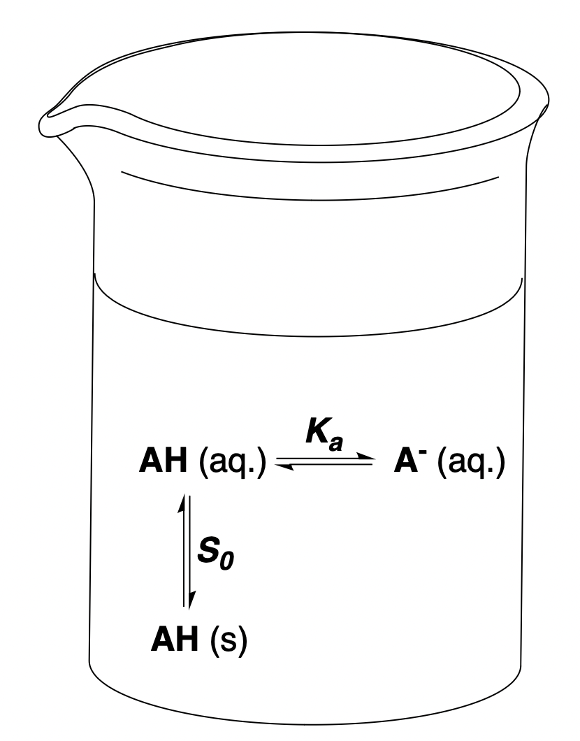
Figure 1: Different equilibria relevant to pH-dependent solubility. The simplified case of a monoprotic acid whose conjugate base is fully soluble is depicted.
For the simple case of a monoprotic acid in an ideal solution without counterions where all charged microstates are perfectly soluble, the full expression for can be written as a function of the solution's , the microscopic acidity constant , and the intrinsic solubility of the monoprotic acid .4,11
Unfortunately, most complex bioactive molecules have multiple ionizable sites, so the above equation does not apply. To generalize this approach to polyprotic acids with coupled sites of (de)protonation, typical in complex drug-like molecules, we reformulate this expression in terms of the "neutral fraction" , the fraction of total material which is in a neutral microstate (i.e. a microstate with 0 net charge).
The aqueous solubility can be obtained by dividing the intrinsic solubility by the neutral fraction, with the two being equal only in the limiting case in which exactly:
This formulation is equivalent to the canonical Henderson–Hasselbalch expression shown above for the case of a monoprotic acid; see Appendix A for more details. Since can be obtained numerically for complex systems with several coupled protonation states, this approach is thus applicable to generic drug-like organic molecules.
In this work, the Starling macroscopic-pKa model was used to compute .9
Dataset
We used the Falcón-Cano "reliable" aqueous-solubility dataset for this work,12 a cleaned, filtered for experimental consistency, and de-duplicated combination of the AqSolDB13 and Cui14 datasets. Each aqueous-solubility measurement was converted to intrinsic solubility using Starling-computed values (assuming a pH of 7.4).
We employed Butina splitting using 1024-bit Morgan fingerprints (with radius 2) to generate train, validation, and test splits.15 In total, we had 12,634 data points divided across 10,043 data points in the train set, 1,256 in the validation set and 1,255 in the test set.
Models
Architectures
We experimented with a variety of modeling approaches in this work. Following Bojan and co-workers,7 we explored the use of atom-level invariant Egret-1 NNP embeddings generated from 3D representations of molecules.16 We generated 3D conformations from SMILES using ETKDG v2 as implemented in RDKit followed by optimization with the MMFF94 forcefield.17–20 We constructed covalent bond graphs of each molecule and used the Egret-1 384-dimensional invariant atom-level features as node embeddings. (Models trained using the entire 1920-dimensional atom-level features had worse performance.)
We used 3 different GNN architectures for solubility prediction: a graph convolutional network (GCN), a graph isomorphism network (GIN), and a graph attention network (GAT). Each GNN has 1 graph convolution layer and 3 subsequent linear layers.21–23
We also fine-tuned the Chemprop-based CheMeleon model from Burns et al.6,24 CheMeleon is a message-passing neural network (MPNN) based on topological molecular-connectivity graphs that was pretrained to predict Mordred molecular descriptors on molecules from PubChem.25
We trained 2 boosted-tree methods, XGBoost and LightGBM, for solubility prediction using Mordred descriptors of molecules as inputs. Boosted-tree methods have previously shown to be effective for solubility prediction.26–28
Finally we used the multiple-linear-regression method ESOL proposed by Delaney.29 This predicts aqueous solubility as the linear combination of simple molecular descriptors: MW, the molecular weight; cLogP, the computed water–octanol partition coefficient; RotB, the number of rotatable bonds; and AromP, the proportion of heavy atoms in the molecule that are aromatic.29 The ESOL method thus has five tunable parameters:
We used Crippen cLogP, as implemented in RDKit, and fit ESOL parameters using an implementation by Pat Walters.19,30,31
Strategies
For each architecture (including ESOL), we investigated four theoretical approaches for solubility prediction:
- Aqueous. We directly predicted the base-10 logarithm of aqueous solubility, .
- Aqueous + fraction. We directly predicted the base-10 logarithm of aqueous solubility, , but additionally added the neutral fraction as an input feature to each model. For ESOL, we added a term for neutral fraction to the multiple linear regression.
- Intrinsic. We predicted the base-10 logarithm of intrinsic solubility, , and created the labels by scaling to with Starling-calculated . We then scaled this prediction back to aqueous solubility.
- Sum. We trained one model to predict the base-10 logarithm of intrinsic solubility, , and then trained a second model to predict the base-10 solubility of the remaining non-intrinsic solubility, .
Several approaches merit further discussion. We trained the "intrinsic" models under the hypothesis that removing the pH-dependent component of aqueous solubility would reduce label variance, making the modeling task simpler. However, we observed that models trained only on intrinsic-solubility labels performed poorly when . To maintain the simplicity of predicting intrinsic solubility while improving performance in the low- regime, we used the "sum" method with the hope of balancing the advantages of both approaches.
We also investigated using Starling to predict the most stable microstate or most stable neutral microstate at pH 7.4 and using these microstates as labels, rather than the default test-set label. These models did not exhibit performance that was statistically significant from models trained on the canonical SMILES labels.
Benchmarking
We benchmarked on three held-out datasets:
- Falcón-Cano External 1, a set of 181 molecules and solubility values reported by Avdeef and co-workers.32 This was employed by Falcón-Cano and co-workers as an external test set.12
- Falcón-Cano External 2, a set of 30 molecules and solubility values from the recent literature that was also employed by Falcón-Cano and co-workers as an external test set.12
- DLS-100, a collection of 100 molecules and solubility values.33 Following Walters,5 we removed any molecules with high similarity to the training set using the same Butina clustering method on Morgan fingerprints as previously stated, resulting in a final test set of 31 molecules.
To additionally assess the ability of our intrinsic-solubility model to predict pH-dependent solubility, we benchmarked against three external pH–solubility curves.34–36
Results
Aqueous Solubility
We began by training 27 models on the Falcón-Cano dataset and evaluating these models on the Butina-split test set. We observed that predicting aqueous solubility was consistently superior to predicting intrinsic solubility—aqueous-solubility-prediction models generally had an of 0.75–0.80 while intrinsic-solubility-prediction models had an of 0.55–0.65 (Figure 2). Adding the neutral fraction as a feature had almost no impact on model performance, and the two-model "sum" strategy also seemed indistinguishable from direct prediction of aqueous solubility.
In contrast, the choice of model architecture had relatively little impact. All deep-learning-based methods (CheMeleon, Egret-1 GNNs, XGBoost, and LightGBM) had very similar performance on this dataset, although ESOL-based models performed significantly worse.
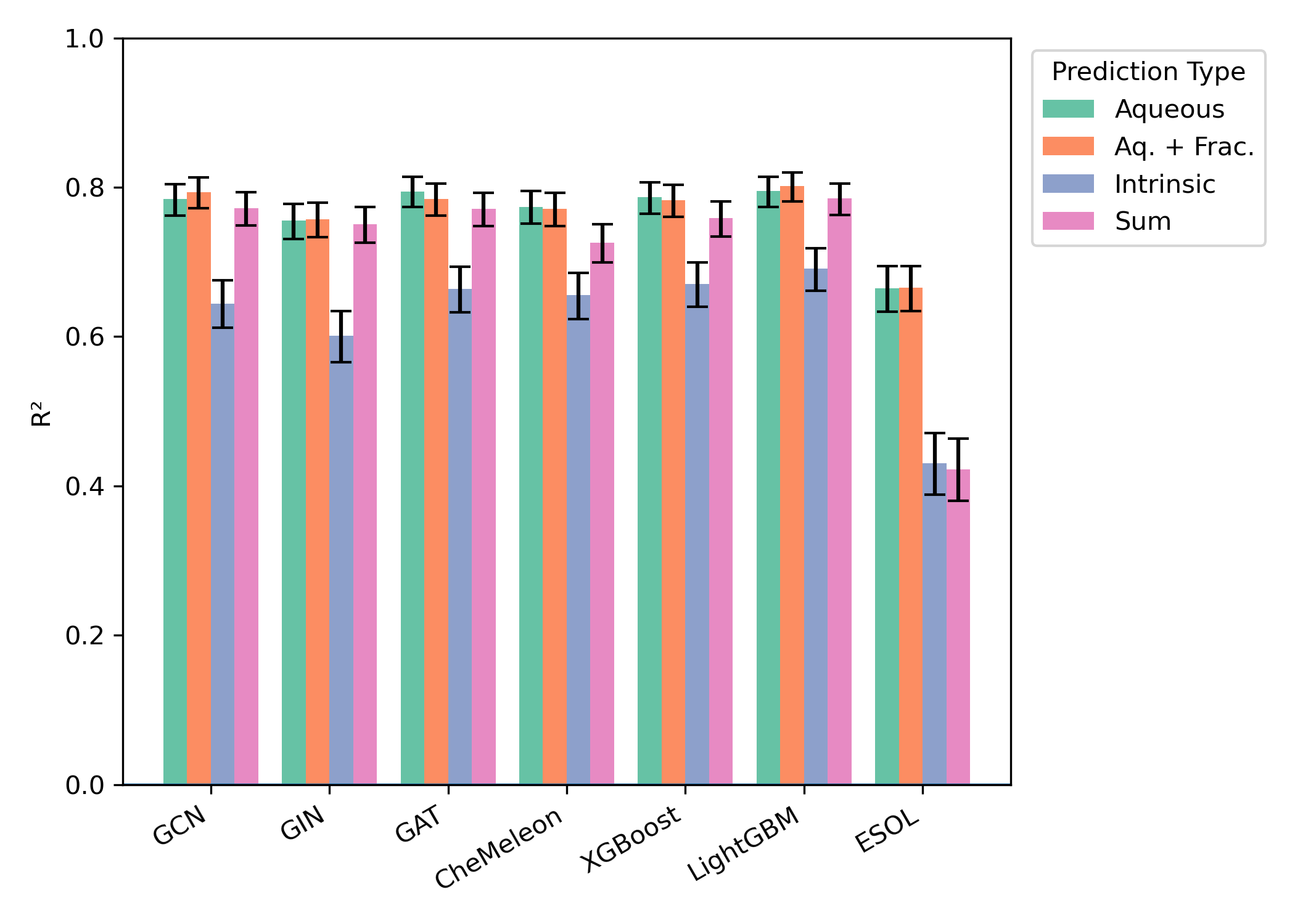
Figure 2: Model performance on the Falcón-Cano test set (1255 molecules). Error bars represent 95% confidence interval for .
External Test Sets
Similar effects were seen across all external test sets: aqueous-solubility prediction with or without consistently outperformed intrinsic-solubility prediction, while the precise choice of model architecture had no consistent impact (Figures 3–5). While the smaller size of the test sets (particularly "External 2" and DLS-100) makes meaningful comparisons hard, there appear to be minimal differences between the different model architectures.
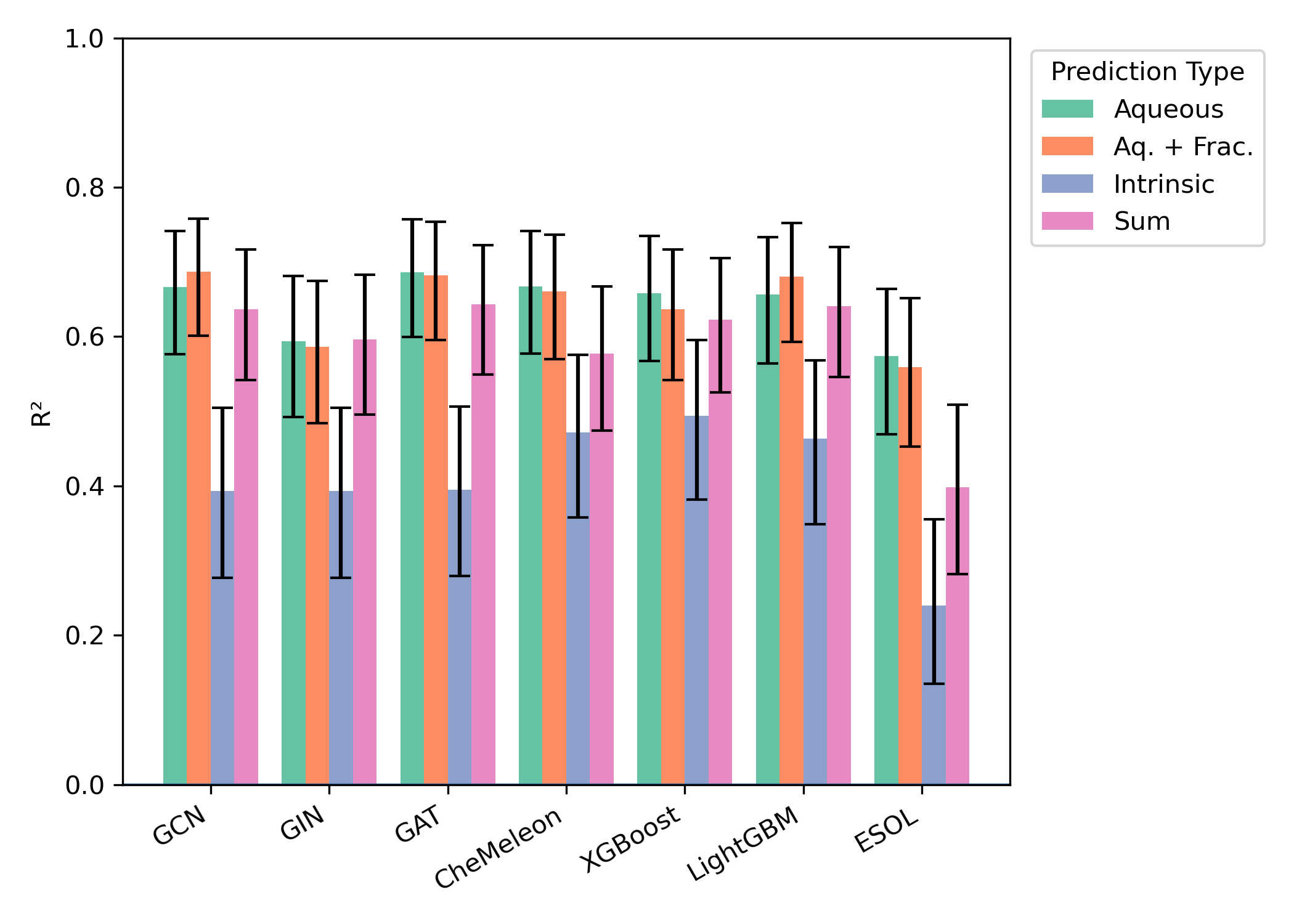
Figure 3: Model performance on the "Falcón-Cano External 1" test set (171 molecules). Error bars represent 95% confidence interval for .
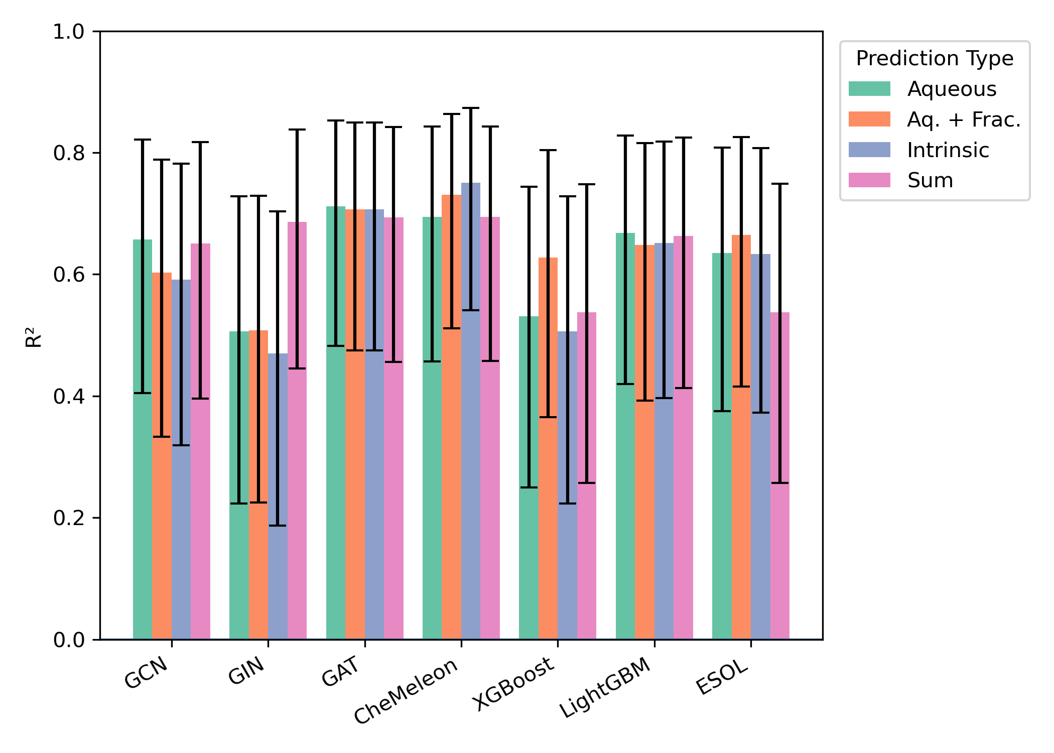
Figure 4: Model performance on the "Falcón-Cano External 2" test set (30 molecules). Error bars represent 95% confidence interval for .
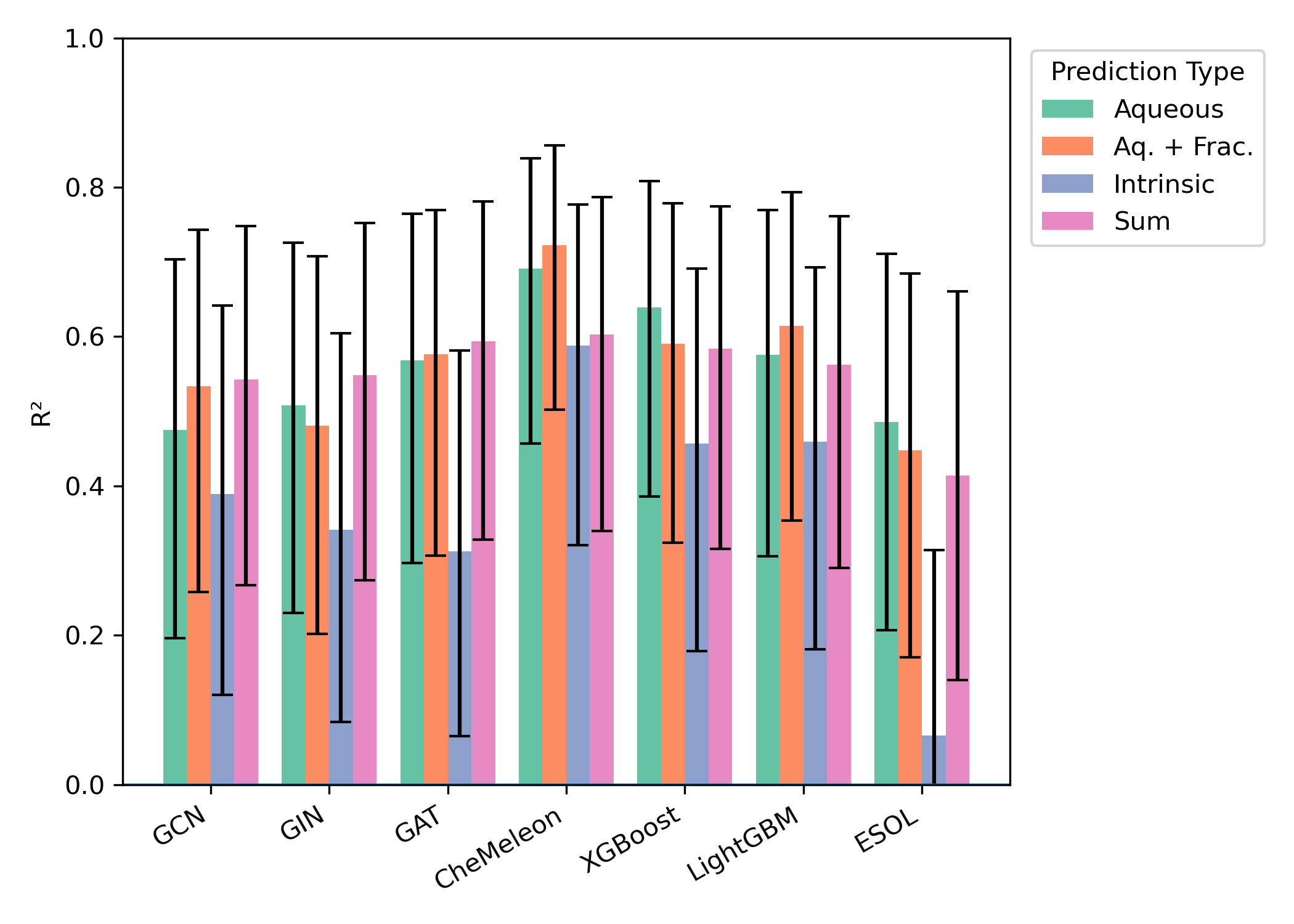
Figure 5: Model performance on the leakage-free subset of DLS-100 (31 molecules). Error bars represent 95% confidence interval for .
Two of the external test sets—"Falcón-Cano External 1" and DLS-100—measure intrinsic solubility, not aqueous solubility. Accordingly, we also investigated direct prediction of intrinsic solubility using the provided intrinsic-solubility models: we were surprised to find that the performance of these models was markedly worse, with typical values between 0.3 and 0.5. While these datasets are often used to benchmark aqueous-solubility models,5,12 the fact that intrinsic-solubility models are worse at predicting intrinsic solubility than aqueous-solubility models is surprising and merits further discussion (vide infra).
Timing
We compared the timing of all methods on both CPU and GPU hardware (Figures 6–7). We found that ESOL was the fastest method and CheMeleon was second-fastest for both hardware configurations.
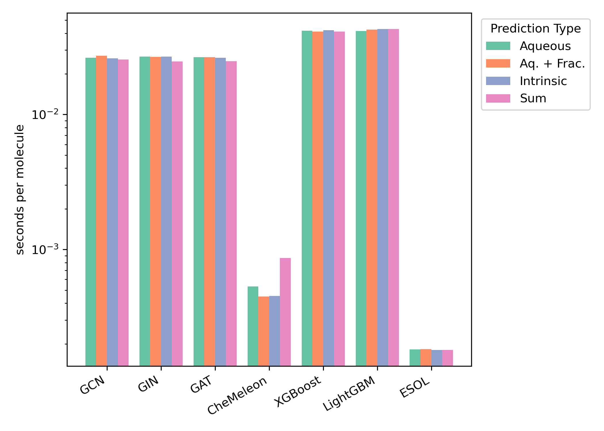
Figure 6: Per-molecule GPU inference time for the Falcón-Cano test set. GPU timing results were obtained using an AMD Ryzen 9 7950X CPU and an Nvidia RTX 4090 GPU. Timings are shown on a logarithmic scale.
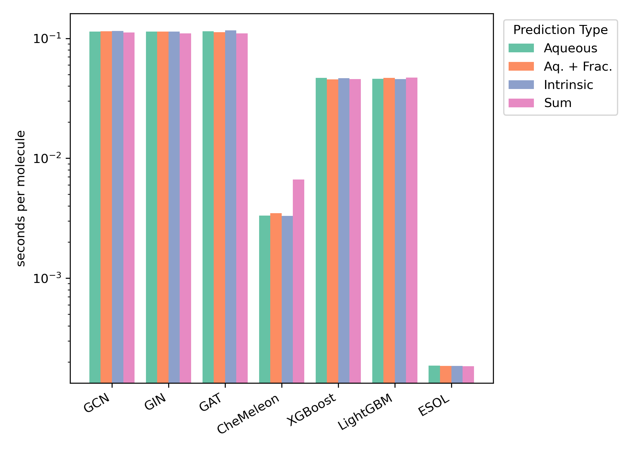
Figure 7: Per-molecule CPU inference time for the Falcón-Cano test set. CPU timing results were obtained using an AMD Ryzen 9 7950X CPU. Timings are shown on a logarithmic scale.
pH-Dependent Solubility
We hypothesized that predicting intrinsic solubility could be used to generate pH-dependent solubility graphs using Starling-predicted values. Since to our knowledge no systematic benchmark set for pH–solubility curves exists, we instead investigated three specific case studies for molecules with well-documented pH-dependent solubility.34–36
Since direct prediction of implicit solubility yielded inferior results to aqueous-solubility prediction (vide supra), pH–solubility curves were generated by (1) predicting aqueous solubility at a neutral pH , (2) converting aqueous solubility to intrinsic solubility by multiplying by the Starling-computed at pH , and (3) multiplying this by to convert back to aqueous solubility at different pH values.
Diprenorphine
Diprenorphine is an opioid-receptor agonist that contains both a weakly basic tertiary amine and a weakly acidic phenol. Accordingly, diprenorphine is least soluble at slightly basic pH values, where neither group is ionized: increasing the pH beyond 9 results in deprotonation of the phenol, while decreasing the pH below 8 results in protonation of the amine (Figure 8).
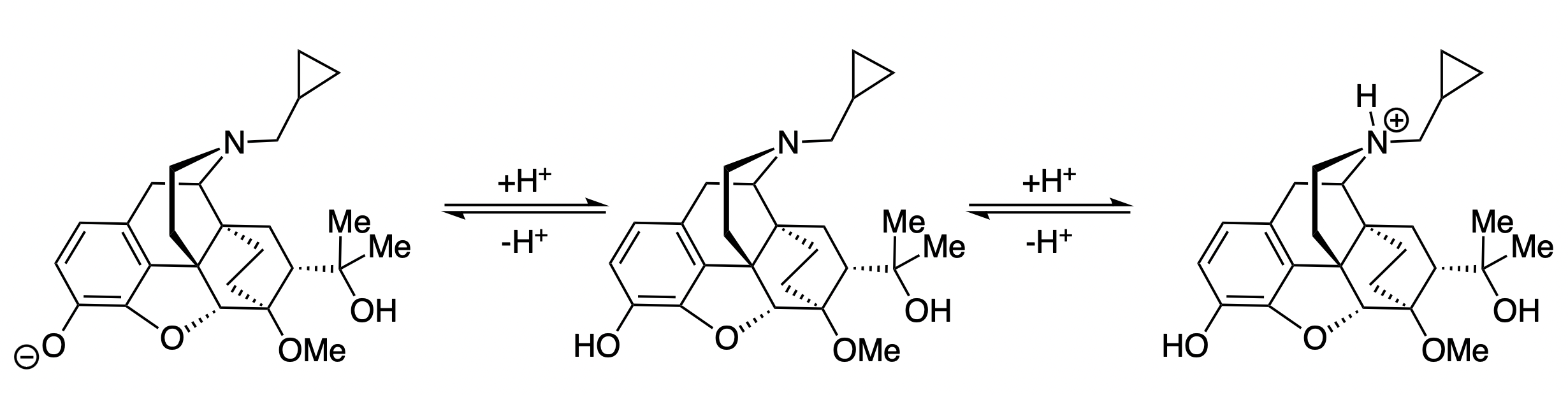
Figure 8: Selected protonation equilibria for diprenorphine.
Predicting with Starling and converting predicted solubility at pH 7.4 to pH-dependent aqueous solubility results in a good match with the experimental pH–solubility curve over most of the pH scale (Figure 9).36 The observed leveling effect at very low pH values is attributed to anion-dependent precipitation, which the authors tentatively ascribe to the hydrochloride salt.36 This non-ideal behavior cannot be modeled within this paper's theoretical framework (vide supra).
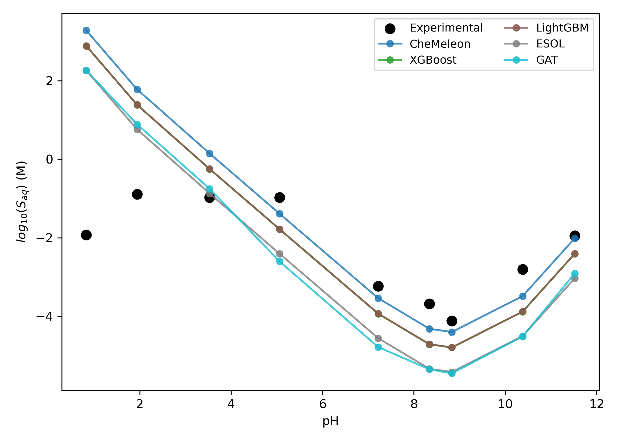
Figure 9: Predicted pH-dependent solubility of diprenorphine. The GCN and GIN models are not shown to reduce visual clutter.
2-Hydroxypropazine
2-Hydroxypropazine is an alkyltriazine known to undergo protonation, which results in increased solubility at low pH values (Figure 10).34 While the various solubility models studied here disagreed on the intrinsic solubility of the neutral species, Starling-predicted correctly predicts a sharp increase in solubility at lower pH values (Figure 11).
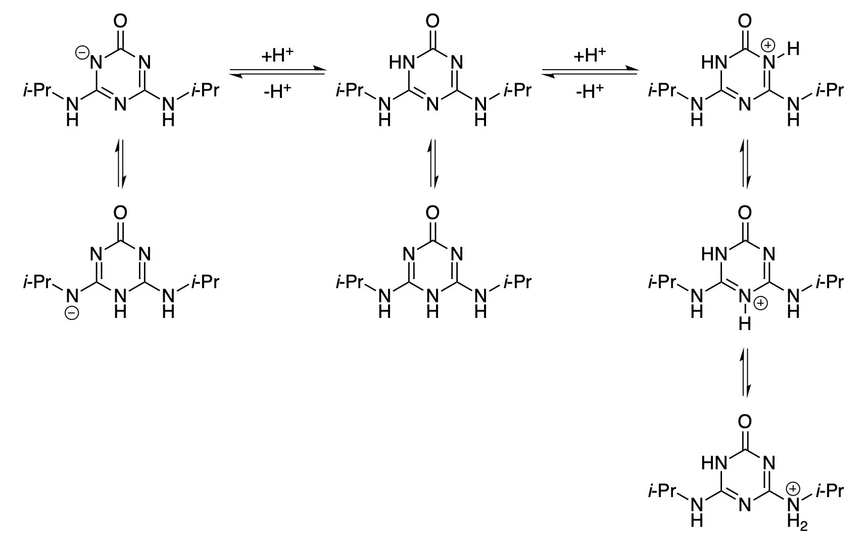
Figure 10: Selected protonation equilibria for 2-hydroxypropazine. Not all potential microstates are shown here.
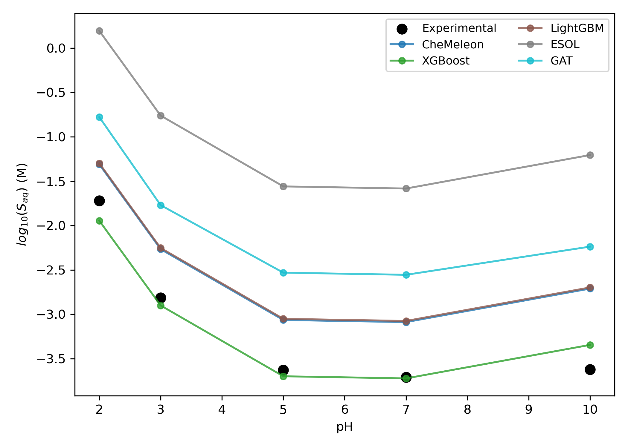
Figure 11: Predicted pH-dependent solubility of 2-hydroxypropazine. The GCN and GIN models are not shown to reduce visual clutter.
Haloperidol
Haloperidol is a common antipsychotic medication that contains a single weakly basic tertiary amine (Figure 12). As with diprenorphine, increasing the acidity of a neutral solution induces a corresponding increase in the solubility of haloperidol, which can be attributed to amine protonation (Figure 13). At low pH values, however, the hydrochloride salt of haloperidol begins to precipitate, so the experimental never exceeds −2 (and even begins to decrease below pH 2, presumably due to the common-ion effect).35
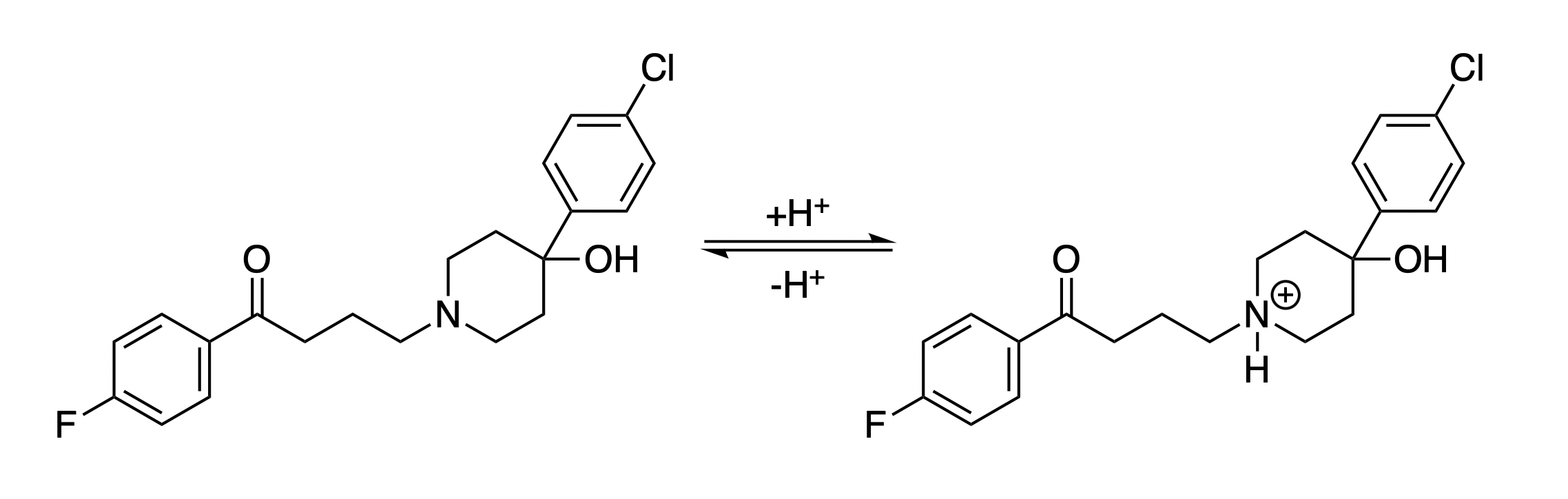
Figure 12: Relevant protonation equilibria for haloperidol.
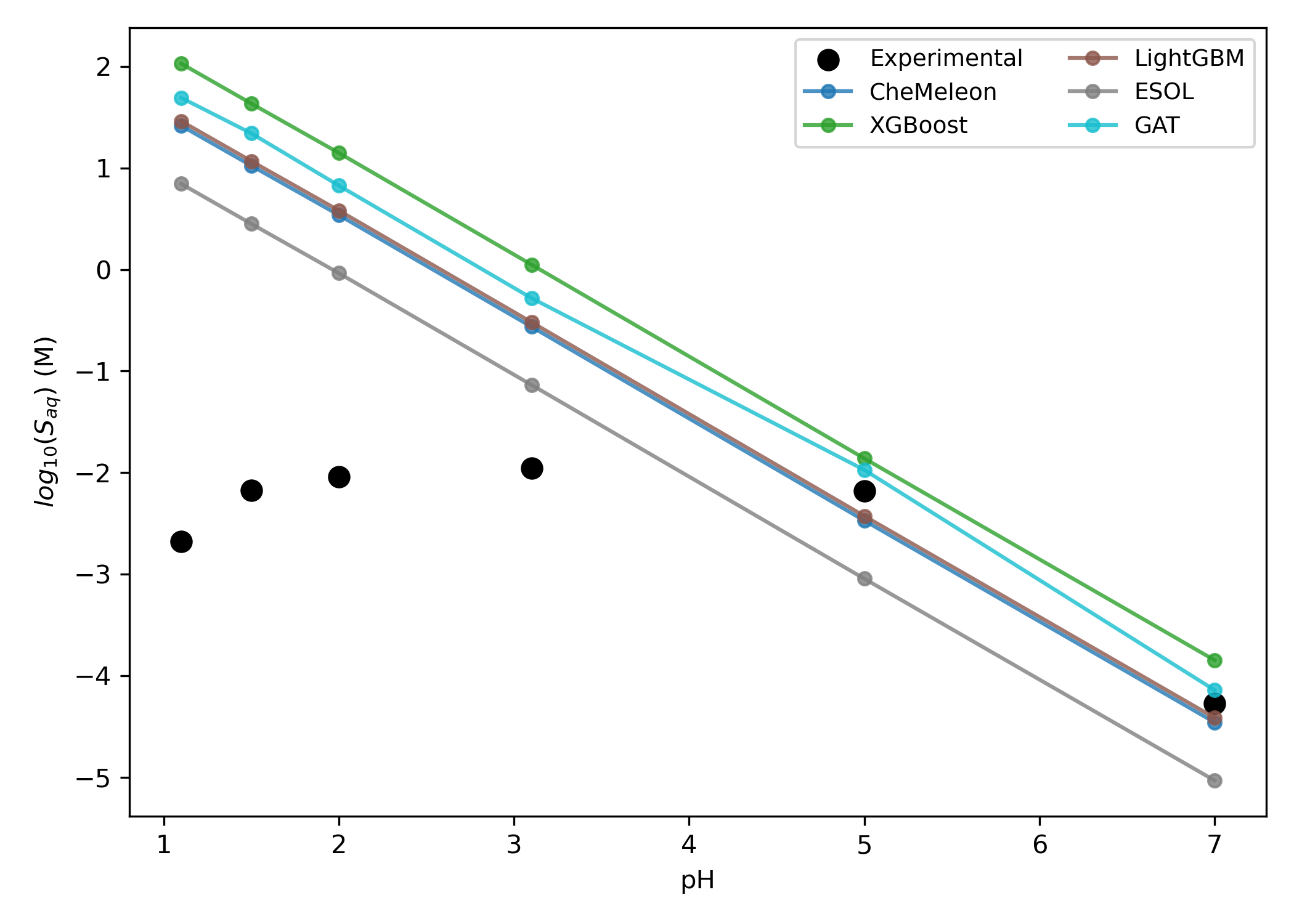
Figure 13: Predicted pH-dependent solubility of haloperidol. The GCN and GIN models are not shown to reduce visual clutter.
Discussion
In this work, we investigated various strategies for combining pretrained molecular representations, macroscopic pKa calculations, and different model architectures, ultimately reporting 28 different combinations of training objective and model architecture. Although the various model architectures and featurization methods we evaluated were strikingly different—ranging from simple multiple-linear-regression models using simple descriptors to complex graph neural networks using the embeddings of neural network potentials—minimal differences in predictive ability were found between the resulting models. This suggests that for current datasets, model expressivity does not limit performance; as found by previous authors, it may be that the intrinsic noise in experimental solubility data constitutes an upper bound on model accuracy.37
In contrast, different theoretical approaches for predicting aqueous solubility produced highly divergent results. The naïve approach of directly predicting aqueous solubility proved superior to predicting intrinsic solubility and converting to aqueous solubility, despite the theoretical advantages of the latter approach. We hypothesize that the failure of intrinsic-solubility approaches arises from inaccuracies in the predicted values—although Starling is a state-of-the-art pKa-prediction model, it still routinely predicts values that are wrong by 0.5–1.0 pKa unit, which can correspond to a 10x difference in the predicted value.9Any inaccuracies in predicting pKa (or in the reported pH of the measurement) can lead to cascading inaccuracies in solubility prediction, as highlighted by Llompart and co-workers:4
The solubility of a compound is highly dependent on its acid-base properties, particularly when the solution pH is within 2 log units of the compound's pKa. Any errors in estimating pKa can lead to large deviations in solubility values.
Since our intrinsic-solubility-prediction models are entirely trained on values generated with Starling-predicted conversions, the error induced by using in silico pKa predictions likely outweighs any benefit of training on . (This also explains why aqueous-solubility models outperformed intrinsic-solubility models on the intrinsic-solubility test sets.) Nevertheless, using to predict pH-dependent solubility gives a good qualitative match with experiment, excepting cases where ion aggregation leads to lower-than-expected solubility.
Our results show that ESOL-based models to be slightly inferior to deep-learning and boosted-tree methods on a variety of benchmarks. Nevertheless, the speed of ESOL makes it an appealing choice for high-throughput virtual screening and other approaches. Since the above workflow involved training ESOL on a large and diverse dataset, we report the following ESOL parameters for black-box usage.
| Descriptor | Coefficients |
|---|---|
| Intercept | 0.261210661 |
| MW | −0.006613884 |
| clogP | −0.741673952 |
| RotB | 0.003451545 |
| AromP | −0.426248404 |
Conclusion
In this work, we investigate a variety of approaches for predicting aqueous solubility and pH–solubility curves, with the goal of leveraging recent advances in pretrained molecular representations and macroscopic pKa predictions to achieve superior performance. Our results demonstrate that relatively simple approaches can do well on these tasks, and that progressing to increasingly complex model architectures and training objectives offers negligible performance improvements. We show that macroscopic pKa calculations can be used to convert solubility under neutral conditions to solubility across the pH scale, allowing for rapid estimation of pH-dependent solubility.
Conflicts of Interest
E.L.M. and C.C.W. are co-founders of the Rowan Scientific Corporation, which is commercializing the CheMeleon-based aqueous-solubility model described here under the "Kingfisher" name.
Acknowledgements
The authors thank Lucas Attia, Jackson Burns, Sanketh Vedula, Pat Walters, & James Yoder for helpful discussions and Ari Wagen & Jonathon Vandezande for editing drafts of this manuscript.
Appendix A: Neutral Fraction-Based Formulation
Let be the population of microstate at a given pH with . We define the neutral fraction as the fraction of all microstate populations that corresponds to microstates with charge equal to 0.
The intrinsic solubility determines the amount of neutral compound that can be dissolved in solution. Since ionization events redistribute material among microstates but do not change the underlying neutral–solid equilibrium, lowering has the effect of increasing the total amount of material that can be dissolved across all microstates. In the case where , half the material is "hidden" from the neutral–solid equilibrium and .
More generally, the aqueous solubility can be obtained by dividing the intrinsic solubility by the neutral fraction, with the two being equal only in the limiting case in which exactly:
This expression can be rearranged to provide a convenient transformation between the base-10 logarithms of aqueous solubility and intrinsic solubility.
Starting from the Henderson–Hasselbalch equation, it is simple to show that the -based approach reproduces the canonical expression for a simple monoprotic acid .4,11
Substituting into the above aqueous–intrinsic transformation equation, we get:
The -based approach reproduces the classic Henderson–Hasselbalch expression but has the advantage of also scaling to complex cases with more than a single ionizable site. While these expressions do not account for the aggregation and non-ideality often observed in aqueous solution, they provide a simple and minimally parameterized way to account for pH-dependent solubility (vide supra).10
Bibliography
- Lipinski, C. A. Drug-like properties and the causes of poor solubility and poor permeability. J. Pharmacol. Toxicol. Methods, 2000, 44, 1, 235–249. DOI: 10.1016/S1056-8719(00)00107-6
- Lipinski, C. A. Poor aqueous solubility—an industry wide problem in drug discovery. Am. Pharm. Rev, 2002, 5, 3, 82–85.
- Lipinski, C. A.; Lombardo, F.; Dominy, B. W.; Feeney, P. J. Experimental and computational approaches to estimate solubility and permeability in drug discovery and development settings. Adv. Drug Delivery Rev., 1997, 23, 1-3, 3–25. DOI: 10.1016/S0169-409X(96)00423-1
- Llompart, P.; Minoletti, C.; Baybekov, S.; Horvath, D.; Marcou, G.; Varnek, A. Will we ever be able to accurately predict solubility? Sci. Data, 2024, 11, 1, 303. DOI: 10.1038/s41597-024-03105-6
- Walters, P. Predicting Aqueous Solubility - It's Harder Than It Looks. Practical Cheminformatics, September 5, 2018. https://practicalcheminformatics.blogspot.com/2018/09/predicting-aqueous-solubility-its.html
- Burns, J.; Zalte, A.; Green, W. Descriptor-based Foundation Models for Molecular Property Prediction. arXiv, June 18, 2025. DOI: 10.48550/arXiv.2506.15792
- Bojan, M.; Vedula, S.; Maddipatla, A.; Sellam, N. B.; Napoli, F.; Schanda, P.; Bronstein, A. M. Representing local protein environments with atomistic foundation models. arXiv, June 16, 2025. DOI: 10.48550/arXiv.2505.23354
- Llinàs, A.; Glen, R. C.; Goodman, J. M. Solubility challenge: can you predict solubilities of 32 molecules using a database of 100 reliable measurements? J. Chem. Inf. Model., 2008, 48, 7, 1289–1303. DOI: 10.1021/ci800058v
- Wagen, C. Physics-Informed Machine Learning Enables Rapid Macroscopic pKa Prediction. ChemRxiv, June 2, 2025. DOI: 10.26434/chemrxiv-2025-t8s9z-v2
- Bergström, C. A.; Avdeef, A. Perspectives in solubility measurement and interpretation. ADMET and DMPK, 2019, 7, 2, 88–105.
- Avdeef, A.; Fuguet, E.; Llinàs, A.; Ràfols, C.; Bosch, E.; Völgyi, G.; Verbić, T.; Boldyreva, E.; Takács-Novák, K. Equilibrium solubility measurement of ionizable drugs–consensus recommendations for improving data quality. ADMET and DMPK, 2016, 4, 2, 117–178. DOI: 10.5599/admet.4.2.292
- Falcón-Cano, G.; Molina, C.; Cabrera-Pérez, M. ADME prediction with KNIME: In silico aqueous solubility consensus model based on supervised recursive random forest approaches. ADMET and DMPK, 2020, 8, 3, 251–273. DOI: 10.5599/admet.852
- Sorkun, M. C.; Khetan, A.; Er, S. AqSolDB, a curated reference set of aqueous solubility and 2D descriptors for a diverse set of compounds. Sci. Data, 2019, 6, 1, 143. DOI: 10.1038/s41597-019-0151-1
- Cui, Q.; Lu, S.; Ni, B.; Zeng, X.; Tan, Y.; Chen, Y. D.; Zhao, H. Improved prediction of aqueous solubility of novel compounds by going deeper with deep learning. Front. Oncol., 2020, 10, 121. DOI: 10.3389/fonc.2020.00121
- Butina, D. Unsupervised Data Base Clustering Based on Daylight's Fingerprint and Tanimoto Similarity: A Fast and Automated Way To Cluster Small and Large Data Sets. J. Chem. Inf. Comput. Sci., 1999, 39, 4, 747–750. DOI: 10.1021/ci9803381
- Mann, E. L.; Wagen, C. C.; Vandezande, J. E.; Wagen, A. M.; Schneider, S. C. Egret-1: Pretrained Neural Network Potentials for Efficient and Accurate Bioorganic Simulation. arXiv, June 11, 2025. DOI: 10.48550/arXiv.2504.20955
- Riniker, S.; Landrum, G. A. Better Informed Distance Geometry: Using What We Know To Improve Conformation Generation. J. Chem. Inf. Model, 2015, 55, 12, 2562-2574. DOI: 10.1021/acs.jcim.5b00654
- Wang, S.; Witek, J.; Landrum, G. A.; Riniker, S. Improving Conformer Generation for Small Rings and Macrocycles Based on Distance Geometry and Experimental Torsional-Angle Preferences. J. Chem. Inf. Model, 2020, 60, 4, 2044-2058. DOI: 10.1021/acs.jcim.0c00025
- RDKit: Open-source cheminformatics. https://www.rdkit.org. 2013–2025.
- Halgren, T. A. Merck molecular force field. I. Basis, form, scope, parameterization, and performance of MMFF94. J. Comput. Chem., 1996, 17, 5-6, 490-519. DOI: 10.1002/(SICI)1096-987X(199604)17:5/6<490::AID-JCC1>3.0.CO;2-P
- Kipf, T.; Welling, M. Semi-Supervised Classification with Graph Convolutional Networks. arXiv, September 9, 2016. DOI: 10.48550/arXiv.1609.02907
- Xu, K.; Hu, W.; Leskovec, J.; Jegelka, S. How powerful are graph neural networks? arXiv, February 22, 2019. DOI: 10.48550/arXiv.1810.00826
- Velickovic, P.; Cucurull, G.; Casanova, A.; Romero, A.; Liò, P.; Bengio, Y. Graph Attention Networks. arXiv, February 4, 2018. DOI: 10.48550/arXiv.1710.10903
- Heid, E.; Greenman, K. P.; Chung, Y.; Li, S. C.; Graff, D. E.; Vermeire, F. H.; Wu, H.; Green, W. H.; McGill, C. J. Chemprop: A Machine Learning Package for Chemical Property Prediction. J. Chem. Inf. Model, 2023, 64, 1, 9–17. DOI: 10.1021/acs.jc01250
- Moriwaki, H.; Tian, Y. S.; Kawashita, N.; Takagi, T. Mordred: a molecular descriptor calculator. J. Cheminf., 2018, 10, 1, 4. DOI: 10.1186/s13321-018-0258-y
- Chen, T.; Guestrin, C. XGBoost: A Scalable Tree Boosting System. arXiv, June 10, 2016. DOI: 10.48550/arXiv.1603.02754
- Ke, G.; Meng, Q.; Finley, T.; Wang, T.; Chen, W.; Ma, W.; Ye, Q.; Liu, T. Y. LightGBM: A Highly Efficient Gradient Boosting Decision Tree. Advances in Neural Information Processing Systems, 2017, 30.
- Li, M.; Chen, H.; Zhang, H.; Zeng, M.; Chen, B.; Guan, L. Prediction of the aqueous solubility of compounds based on light gradient boosting machines with molecular fingerprints and the cuckoo search algorithm. ACS Omega, 2022, 7, 46, 42027–42035. DOI: 10.1021/acsomega.2c03885
- Delaney, J. S. ESOL: Estimating Aqueous Solubility Directly From Molecular Structure. J. Chem. Inf. Comput. Sci., 2004, 44, 3, 1000–1005. DOI: 10.1021/ci034243x
- Wildman, S. A.; Crippen, G. M. Prediction of Physicochemical Parameters by Atomic Contributions. J. Chem. Inf. Comput. Sci., 1999, 39, 5, 868–873. DOI: 10.1021/ci990307l
- Walters, P. solubility. 2018. DOI: https://github.com/PatWalters/solubility,
- Avdeef, A. Prediction of aqueous intrinsic solubility of druglike molecules using Random Forest regression trained with Wiki-pS0 database. ADMET and DMPK, 2020, 8, 1, 29–77. DOI: 10.5599/admet.766
- McDonagh, J. L.; Nath, N.; De Ferrari, L.; Van Mourik, T.; Mitchell, J. B. Uniting cheminformatics and chemical theory to predict the intrinsic aqueous solubility of crystalline druglike molecules. J. Chem. Inf. Model, 2014, 54, 3, 844–856. DOI: 10.1021/ci4005805
- Ward, T. M.; Weber, J. B. Aqueous solubility of alkylamino-s-triazine as a function of pH and molecular structure. J. Agric. Food Chem., 1968, 16, 6, 959–961. DOI: 10.1021/jf60160a034
- Li, S.; Wong, S.; Sethia, S.; Almoazen, H.; Joshi, Y. M.; Serajuddin, A. T. Investigation of solubility and dissolution of a free base and two different salt forms as a function of pH. Pharm. Res., 2005, 22, 4, 628–635. DOI: 10.1007/s11095-005-2504-z
- Völgyi, G.; Marosi, A.; Takács-Novák, K.; Avdeef, A. Salt solubility products of diprenorphine hydrochloride, codeine and lidocaine hydrochlorides and phosphates–Novel method of data analysis not dependent on explicit solubility equations. ADMET and DMPK, 2013, 1, 4, 48–62. DOI: 10.5599/admet.1.4.24
- Attia, L.; Burns, J. W.; Doyle, P. S.; Green, W. H. Data-driven organic solubility prediction at the limit of aleatoric uncertainty. Nat. Commun., 2025, 16 , 1, 1–10. DOI: 10.1038/s41467-025-62717-7