Guessing Transition States
by Jonathon Vandezande · Jun 5, 2025
A transition state (TS) is the highest energy point on the minimum energy path between reactants and products. Finding an accurate TS is incredibly useful in reaction modeling because the energy difference between the TS, reactants, and products determines the rate of a reaction. Due to the high-dimensional space that molecules exist in, locating these transition states is non-trivial for all but the simplest reactions.
Often, transition states are found by first locating an approximate or "guess" TS. These guess transition states can be optimized with second-order Newton methods utilizing the calculation of a Hessian (matrix of mixed second derivatives). For this to work, the guess must be close to the actual TS, and it is often unclear where to begin when finding a guess. This blog surveys various methods for generating guess transition states.
Note: this post adopts concepts from our previous blog post "Reactions from the Bottom Up," which we advise you to review before continuing.
Before we jump into guess-TS-finding methods, we'll start by defining a few terms:
- Tangent (to a curve): vector at a point on a curve that points along the curve.
- Normal space (to a curve): space orthogonal to the curve tangent.
- Minimum energy path (MEP): path connecting reactants and products that at every point minimizes the energy in all directions normal to the curve (a geodesic connecting reactants and products).
- Trial direction: a direction in coordinate space used as a guess for the direction of the MEP.
- Reaction channel: area around the MEP.
- Saddle point: a point where the derivative is zero in every direction, but it is not a local maximum or minimum (chemistry mostly deals with first-order saddle points, where the potential energy surface curves upward in all dimensions except one, in which it curves downward).
- Hessian: matrix of mixed second derivatives. Diagonalizing it shows the curvature at a point. Diagonalizing the Hessian evaluated at a 1st-order saddle point will result in a single negative eigenvalue.
Synchronous Transit (Interpolation)
Many TS guess methods attempt to use a surrogate for the MEP to constrain the search and optimization. These surrogate MEPs avoid calculating expensive Hessians, thereby reducing the complexity of searching for saddle points on a high-dimensional surface. Interpolating the coordinates between reactants and products often provides a reasonable surrogate for the MEP and is frequently the easiest way to get started.
Linear Synchronous Transit (LST)
Perhaps the simplest method for guessing the TS is to naïvely interpolate between the reactants and products and then find the highest energy point along this path. This method is called Linear Synchronous Transit (LST). It often produces a poor guess for the TS, with multiple imaginary frequencies. For the linear H + H2 PES, a linear geometric interpolation between (0.75, 1.7) and (1.7, 0.75) (the dotted blue line in Figure 1 below), passes through a region of very high energy (a region rarely accessed via normal atomic motion).
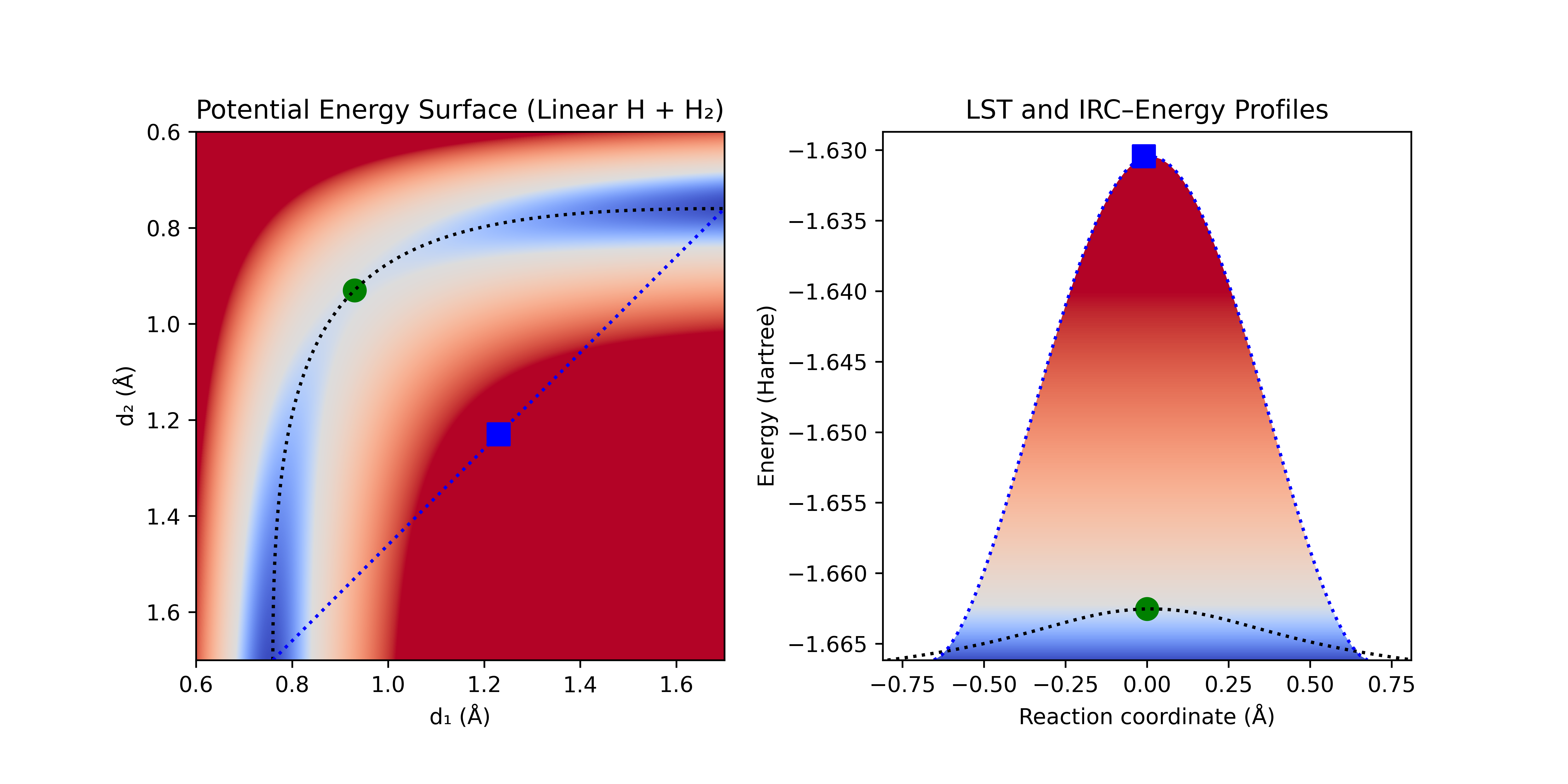
Figure 1: Linear H + H2 PES with naïve interpolation [blue dotted line], true IRC [black dotted line], LST guess for TS [blue square], and true TS [green dot].
The interpolation in Figure 1 is done in internal coordinate space. Things can become very problematic when done in Cartesian space, with unrelated bonds forming and breaking during the interpolation. Various methods have been developed to improve this, including image dependent pair potential (IDPP, based on interpolated pairwise distances) and sequential IDPP (S-IDPP, similar to NEB (discussed later)). Things can get even worse for systems like the isomerization of H–C≡N → C≡N–H (TS structure). The true isomerization pathway has the hydrogen go around the central C≡N, but linear interpolation would cause it to pass through the C≡N, leading to unphysical geometries with atoms stacked on top of each other.
Quadratic Synchronous Transit (QST)
LST can be improved by allowing alternative interpolations of the coordinates and then optimizing normal to the interpolation. Quadratic synchronous transit (QST) uses quadratic interpolation of the coordinates to provide greater flexibility for possible geometries. A constraining curve is constructed from this quadratic interpolation of the coordinates, and the highest point along this curve is located. The geometry at this peak is then optimized normal to the curve. If the resulting geometry is not a TS, the process is repeated until convergence: a new curve is constructed through the reactants, products, and this latest TS guess, the maximum is found along this new curve, and then the geometry is optimized normal to the curve at the maximum. The curve provides a simple surrogate for the reaction path, while constraining the geometry to the peak of the curve provides a simple method to avoid collapse to the reactants or products.

Figure 2: Quadratic Synchronous Transit (QST) with LST initial guess. QST constraining curves [dotted blue lines] and direction of optimization in normal space [black arrows].
Since a linear interpolation is often a poor starting point, a TS guess is typically added to stretch the initial constraining curve (QST3). If a poor initial TS guess is chosen, QST3 can still often recover (though it may require more iterations). Figure 3 shows such a case. After a poor initial guess and finding the local maximum along the profile (red square), optimization in the normal space causes the local maximum to collapse and the optimization along the curve finds the global maximum along the curve (blue square). From here the optimization follows as in Figure 2 to locate the TS (green circle).
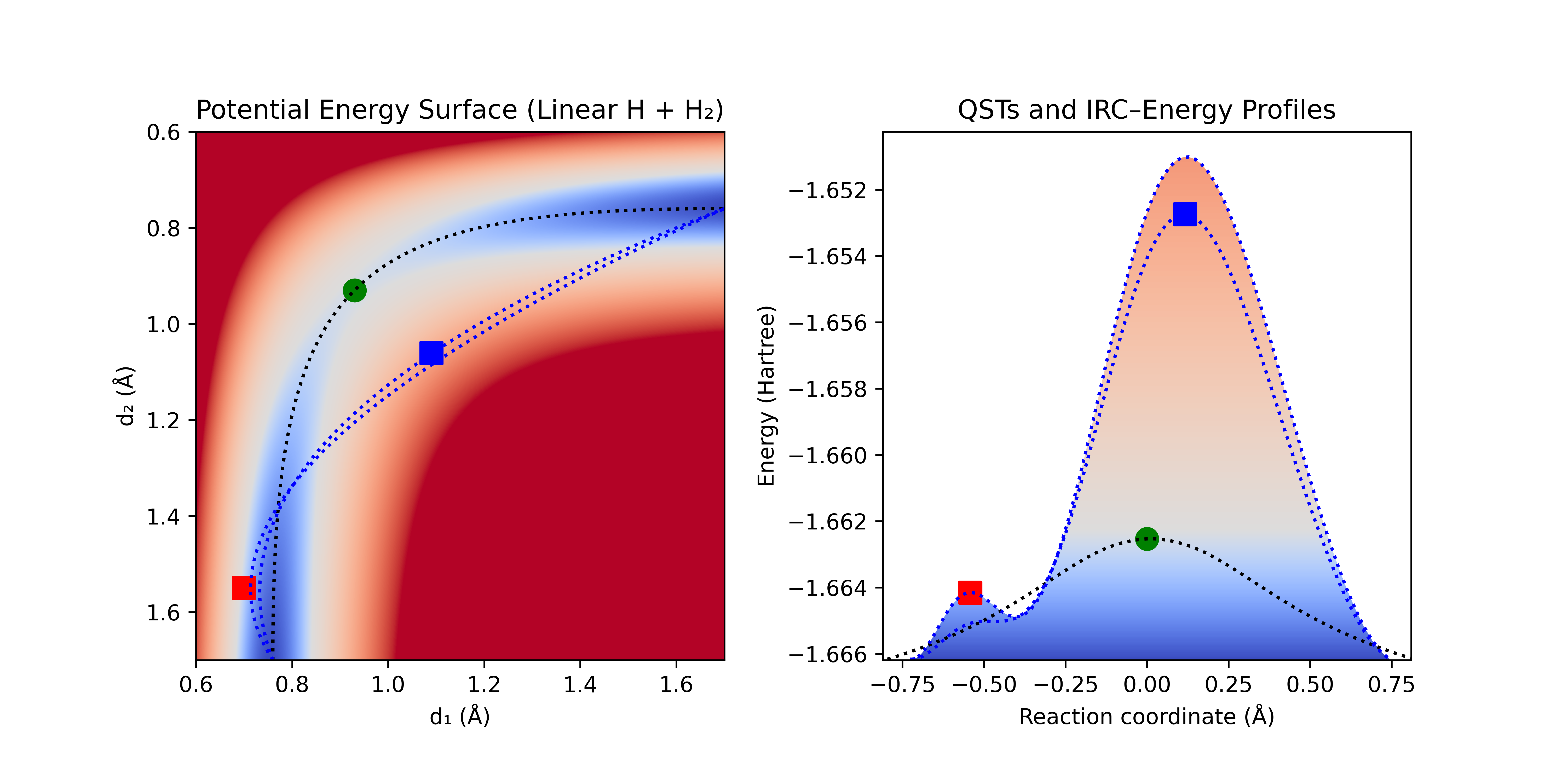
Figure 3: Quadratic synchronous transit (QST3) with poor initial guess [red square] showing the ability of QST3 to recover.
QST3 is a very robust method, but it can still struggle for a variety of reasons:
- Poor choice of initial geometries (e.g. van der Waals complex that is not aligned with the reaction)
- Poor choice of coordinates
- Poor TS guess (e.g. linear interpolation of H–C≡N → C≡N–H)
- Internal coordinates that can't reasonably be approximated by a parabola across the IRC (e.g. a coordinate increases, then decreases, then increases)
- Multi-step reactions
QST3 is often a good choice if you have a guess for the TS that looks plausibly like the true TS, even if it is far from the true TS. However, the requirement of a guess TS to avoid high energy regions makes it difficult to use QST3 in an automated fashion for TS screening.
Elastic Band (EB)
Elastic band (EB) methods act as though an elastic band has been stretched between the starting and ending structure, and is then allowed to relax away from regions of high energy. It starts by placing nodes along a guess pathway (EB literature usually uses the term "image" for nodes). Nodes are coupled via spring-like interactions, with forces that are attractive or repulsive based on the distance between nodes. Nodes are then all optimized subject to this constraint. This allows the nodes to "stretch" the elastic band away from regions of high energy, while avoiding the collapse of the nodes to the reactants and products.
Nudged Elastic Band (NEB)
Early EB methods suffered from "corner-cutting" due to spring forces pulling the nodes off the minimum energy path (MEP). To avoid this, nudged elastic band (NEB) decomposes the forces from the gradient of the PES and the spring force into components tangent and normal to the path. It then only uses the tangent component of the spring force to attract the nodes, and only the normal component of the gradient to optimize the node (termed "nudging"), similar to QST3 and GSM. The spring forces thus control the spacing between the nodes, but have minimal effect on the path direction.
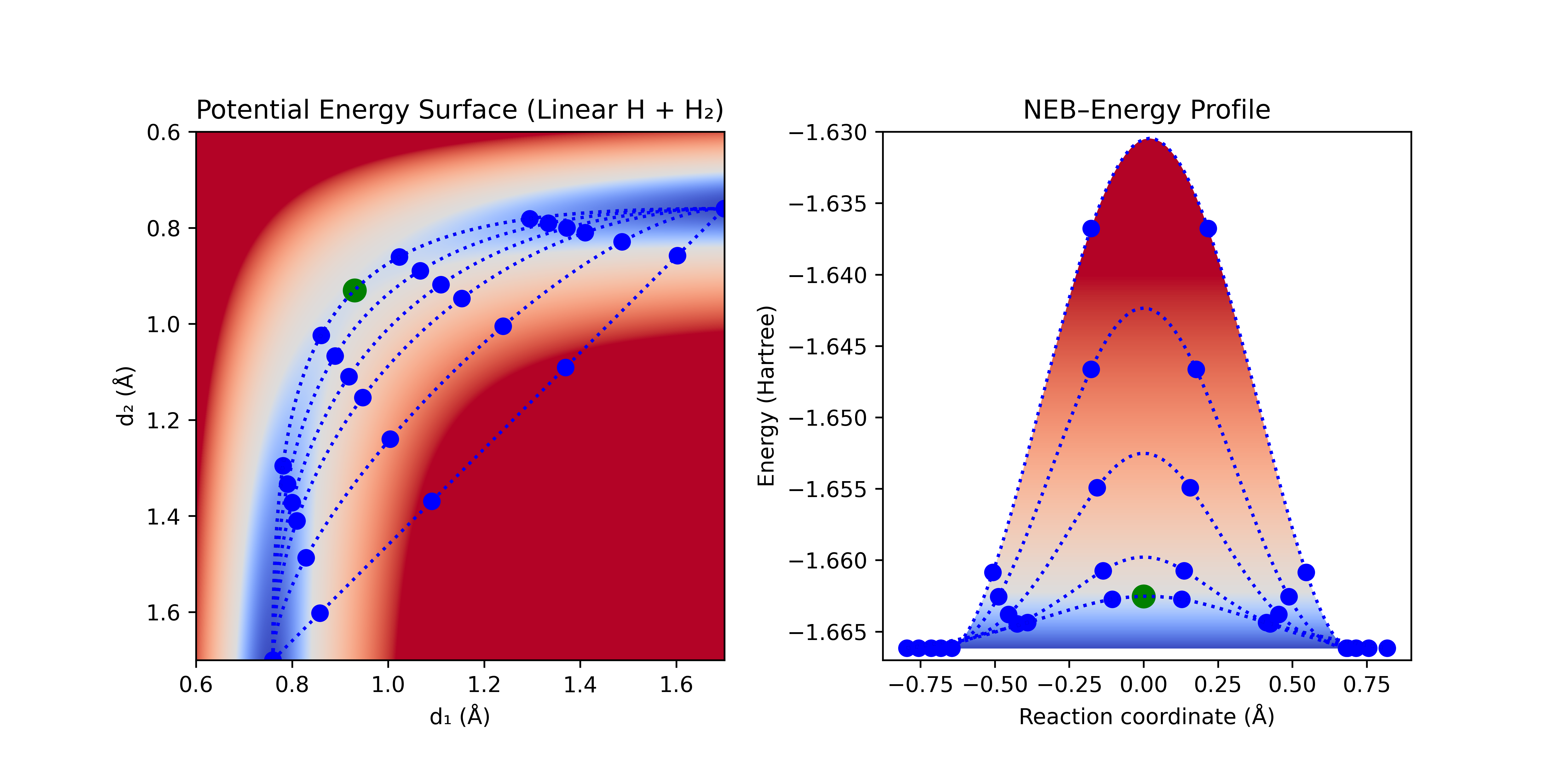
Figure 10: NEB progression. An initial guess for the path is generated, and nodes are optimized normal to the path while being attracted to each other with spring forces along the path.
With enough nodes, NEB will often converge to a close approximation of the MEP, and can even find reaction paths that include intermediates. However, with the computational cost increases with the number of nodes, and too many nodes can lead to kinks in the path.
Climbing-Image Nudged Elastic Band (CI-NEB)
In standard NEB, the TS is often between two nodes, and thus an interpolation between these nodes is needed to generate a guess TS (which in turn needs to be optimized to the true TS). CI-NEB adds a correction similar to QST; the highest energy node is taken as a guess for the TS and is constrained by the nodes on either side. Tangent to the band, the node climbs the gradient, while being minimized normal to it. Since the nodes in NEB are much closer to the TS than the reactants and products, this minimizes many of the issues seen with QST.
Channel Following
Naïve Channel Following
Reaction channels are often aligned with vibrations in the reactants and products. Naïve reaction channel following chooses the lowest-energy vibrational modes as trial directions and follows them until a barrier is surmounted. A linear interpolation of the mode may work for simple transition states (such as rotational barriers), but will often run into the same problems as LST. Alternatively, the Hessian (or its approximation) can be recomputed at each step and the mode that is most similar to the mode used in the previous step can be followed iteratively until the barrier is surmounted.
This method works well for small molecules with limited degrees of freedom, and can precisely approximate an MEP with small step sizes. However, the need to calculate an initial Hessian and consistently update it is prohibitive for large systems, and can easily be misled by irrelevant low-frequency modes in the initial selection or while attempting follow the path.
Dimer Method
An improvement on naïve coordinate following is the dimer method. It estimates the local curvature by using a pair of geometries separated by a small distance in coordinate (thus avoiding the computation of a Hessian). The method rotates the line connecting the two geometries (the "dimer") around its midpoint to find the direction that most reduces the sum of the energies of the dimer. (This rotation happens in the high-dimensional coordinate space—not a literal rotation of the molecule in 3D space.)
This minimization aligns the dimer with the direction of lowest curvature (assuming a small separation distance and a locally quadratic surface). A step is then taken along this vector in the uphill direction, and the process is repeated until the pair starts going downhill (indicating that a saddle point was reached). This method avoids the need for a Hessian, and works well for following channels, but can get lost in systems with multiple, low-energy modes (thus it is most common in periodic DFT calculations where most of the surface is either fixed or has stiff vibrational modes).
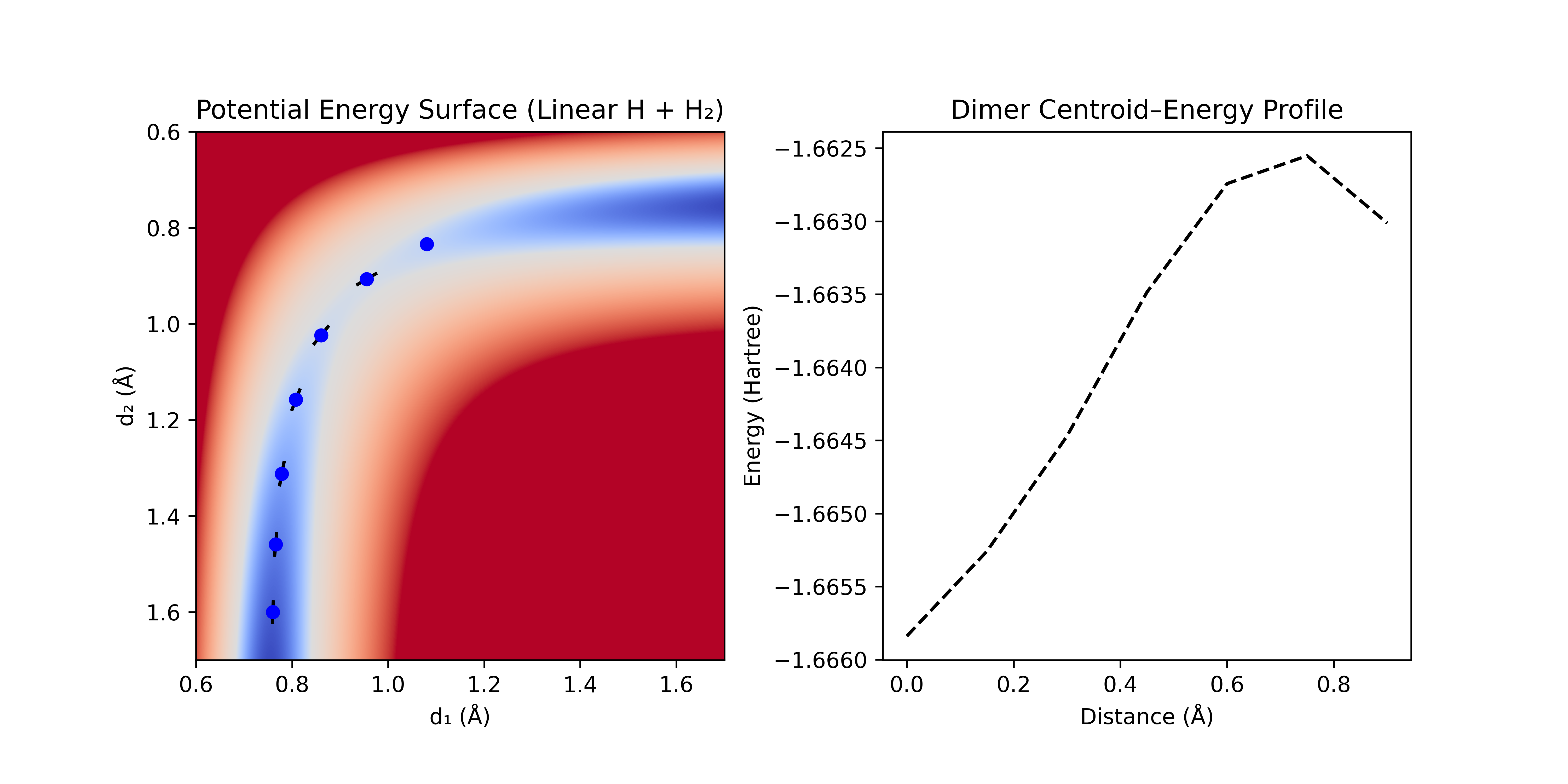
Figure 4: Dimer method following the path of lowest curvature. The dimer [black bars] is rotated around the pivot point [blue dots] until the lowest total energy is achieved. An uphill step is taken along this direction and the process is repeated until the barrier is crossed.
Coordinate Driven
Constrained Optimization
The simplest form of coordinate-driven TS-guess generation is to just guess the local geometry of the transition state, fix all coordinates (bonds, angles, and/or dihedrals) involved in the transition mode, and optimize all other coordinates. While rarely useful for novel transition states, this is commonly used if a TS has been found for a similar reaction, and the R-groups just need to be swapped out (e.g. Figure 5). This can also be useful when combined with QST3 to help hold the system near the TS or metadynamics-based transition state conformer search (discussed later).
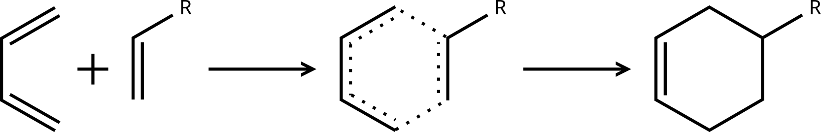
Figure 5: Diels–Alder reaction with an R-group to be replaced
Coordinate Scanning
An alternative to interpolation for generating new transition states is to simply scan across a coordinate (or set of coordinates) and let all other coordinates relax (e.g. for H + H2, just pull the two hydrogens together and let the other one float off when it wants). This allows the system to avoid regions of very high energy or atom clashing that can be seen in interpolation-based methods. It works passably well for single bond-breaking/forming reactions, where the coordinate reasonably approximates the IRC, but performs poorly when the coordinates involved change throughout the reaction. H + H2 involves an initial bond-formation, followed by bond-breaking, and thus is difficult to describe with a single coordinate; choosing a single coordinate to drive it will often cause an atom to float off into space.
Concerted scans over multiple bond formations can generate more complex transition states (e.g. Diels–Alder reactions). However, for mixed formation/dissociation (e.g. H + H2 bond formation/breaking), this requires careful matching of coordinates. Alternatively, a 2D (or higher-dimensional) scan can be performed across multiple coordinates to find a good guess for the TS (as in a More O'Ferrall–Jencks plot), but this can become prohibitively expensive for larger reactions where a large number of points must be calculated. Coordinate scanning is often relied upon for generating transition states, but only because more robust methods are not available in every package.
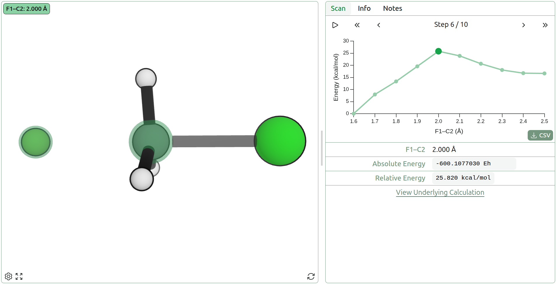
Figure 6: Coordinate scan of F––C bond distance using AIMNet2 in the SN2 reaction of F– + CH3Cl → FCH3 + Cl– (view on Rowan)
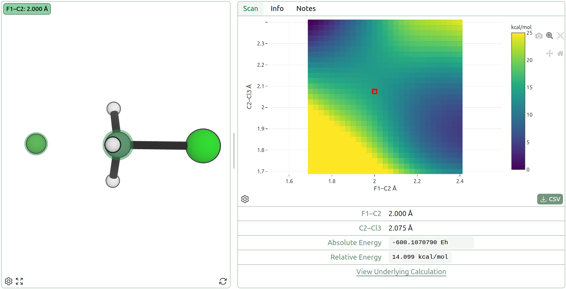
Figure 7: 2D coordinate scan of F––C distance and C–Cl– distance using AIMNet2 in the SN2 reaction of F– + CH3Cl → FCH3 + Cl– (view on Rowan)
Growing String Method (GSM)
Growing string methods extend the coordinate-driven paradigm by starting from the reactant geometry (and product geometry for double-ended GSM) and perturbing it along a guess for the reaction coordinate. Successive nodes are added to the path and optimized to fall along the minimum energy path, while being "held up" by the prior nodes.
Single Ended
Single-ended GSM starts from an equilibrium structure and creates a perturbed geometry along a trial direction for the reaction path (GSM literature refers to each of these geometries as a node). Successive nodes (geometries) are added to the path along the tangent (often defined by a cubic spline of existing points), and then optimized in the normal space of a cubic spline connecting the points (i.e. in all directions not along the path). This process is repeated until the path starts going downhill, indicating that the transition state has been passed (as with the dimer method). Traditional GSM methods optimize every node after each new node is added, while frozen string methods optimize only the frontier nodes and often only perform a few optimization steps instead of attempting to achieve a fully optimized geometry.
With small enough step sizes, single-ended GSM can follow the local contours of the PES, while avoiding collapse back to the reactants. However, if a poor guess is chosen for the initial perturbation, it may produce an undesired TS (e.g. methyl rotation). Single-ended GSM is particularly useful for exploration of possible reactions on the PES when the desired products are unknown.

Figure 8: Single-ended GSM. A step [dotted blue line] is taken tangent to the path, and then optimized normal to the path [black arrows]. This process is repeated until the barrier is crossed.
Double Ended
Double-ended GSM is similar to single-ended GSM, but a string is grown from both the reactants and products. Starting from optimized reactant and product geometries, nodes are placed near each endpoint and perturbed either towards the opposite node, or along a predicted initial coordinate (the latter avoids the H–C≡N isomerization problem discussed in the LST section). Successive steps are taken in the direction of the opposite node, and then all nodes are optimized in the normal space of the path. This process is repeated until the two strings meet.
This method avoids the generation of an initial guess pathway, avoiding some of the pathological problems associated with interpolation methods. This method is robust to intermediates, and as in single-ended GSM, it can be accelerated by freezing all but the newest nodes in the path during the optimization step.

Figure 9: Double-ended GSM with linear synchronous transit interpolation. A step [dotted blue line] is taken along the linear interpolation towards the other end, and then optimized normal to the step [black arrow]. This process is repeated until the ends meet.
Metadynamics
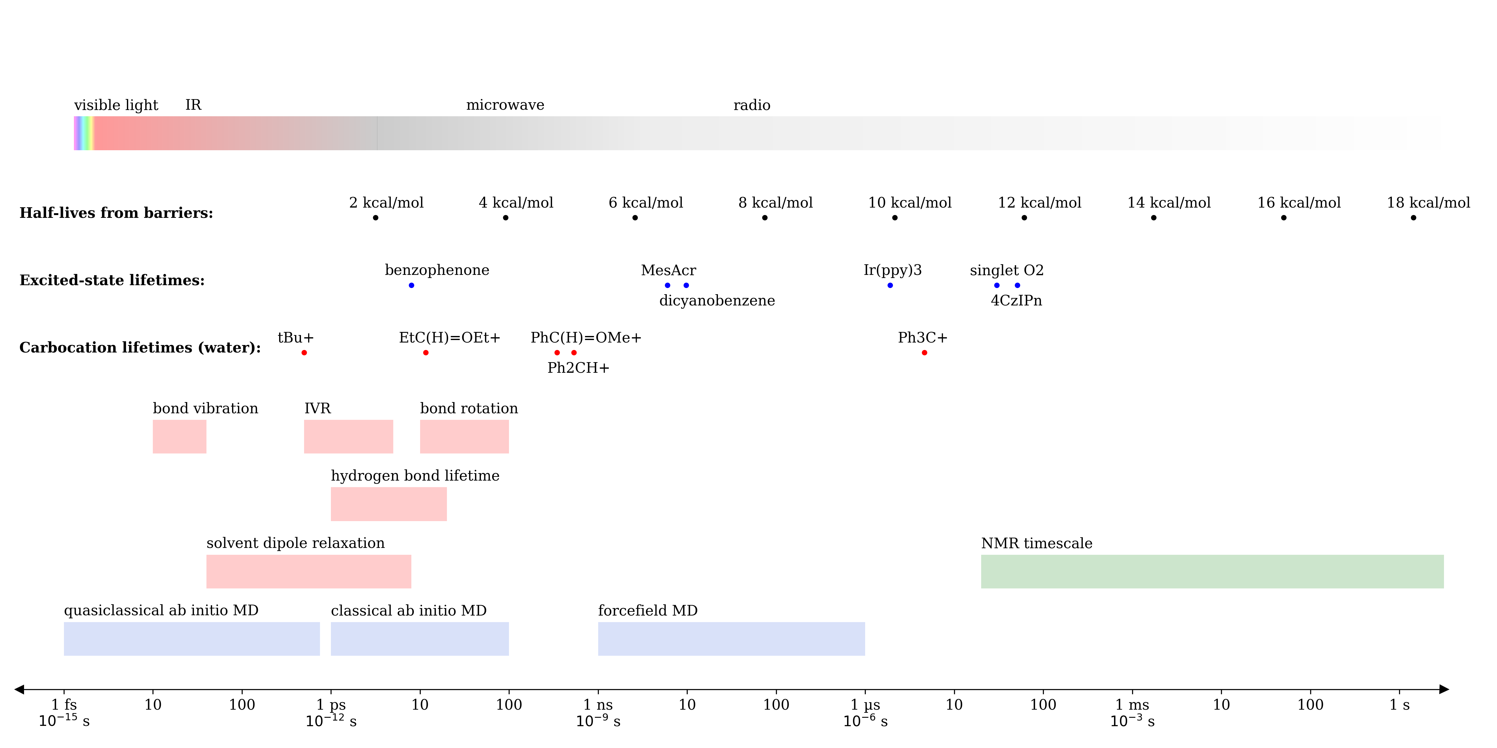
An alternative method to finding transition states via optimization, channel following, or constraining to a path/band, is to run molecular dynamics (MD) and observe the transitions happen between reactants and products. Traditional MD would be too slow, as reactions are incredibly rare compared to the time-steps (time-steps are on the order of femtoseconds, while the half-life of a 10 kcal/mol barrier is ≈1 µs and a 20 kcal/mol barrier is ≈1 s, see this helpful graphic from Corin Wagen). To accelerate the reactions, a biasing potential is applied that pushes the current system away from the reactants and any part of the PES that has already been traversed (and towards the products if known). This is similar to water slowly filling up a lake, looking for the lowest point to spill over the dam that holds it back (the optimal biasing force and collective variables are an open question).
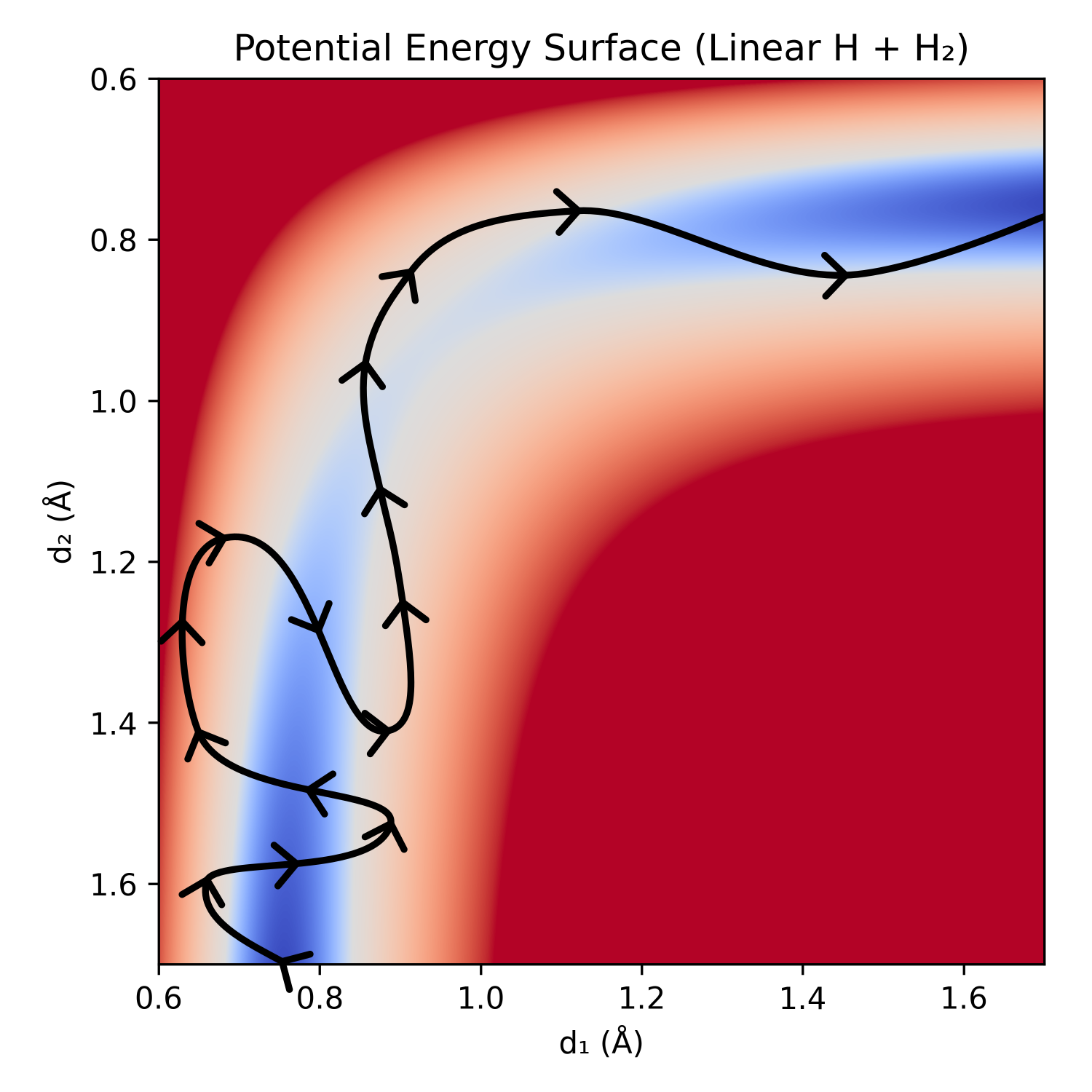
Figure 10: Simplified depiction of a metadynamics exploration of the linear H + H2 potential energy surface.
This is useful when there isn't an obvious path between the reactants and products, when simple interpolation between coordinates enters regions of incredibly high energy (e.g. H–C≡N → C≡N–H), or when the desired product is unknown.
Metadynamics-based reaction-path methods require a surrogate for the partition space to determine when a reaction has occurred. For many reactions this can just be the determination if a specific bond has formed or broken. Every time the dividing surface between the partition spaces is crossed, a reaction is deemed to have occurred. If this process is repeated numerous times, a rate can be estimated (this is exact in the limit of no biasing potential and an infinite number of samples). Alternatively, the path can be traced back across the dividing surface to find a guess for the minimum energy path. This path can then be fed into another TS finding algorithm such as CI-NEB to generate the true TS.
Metadynamics methods can be incredibly expensive due to the large number of steps involved, and often require approximate methods such as the semiempirical GFN2-xTB or a neural network potential (NNP) to run in an acceptable amount of time. They also have difficulties with multi-step reactions, as typically only one dividing surface is defined.
Conformer Searching TSs
There are often multiple unique paths a reaction could pass through (such as concerted vs sequential reactions) and multiple conformers that the reactants could be in at the TS. While the above methods can generate transition states, they cannot guarantee the lowest energy transition state has been found, nor can they account for the entropy of multiple low-lying transition states. Ideally, there would be a method that can perform a conformer search only within the N–1-dimensional dividing surface separating reactants and products. However, since precisely defining this hypersurface is difficult, it is instead common to define a proxy (e.g. a set of bond distances or angles) that is fixed (or at least strongly constrained) while a conformer search is performed on all other coordinates. This then produces guesses that can be input into TS optimization for further refinement.
The most common form of this type of search is to use constrained metadynamics to search out the possible conformers. Snapshots of these dynamics can be taken, individually optimized (with the TS defining constraints), and deduplicated to obtain guesses for TSs. The guesses are then refined using a TS optimization method to obtain other possible transition states. The energy of the dividing surface can then be reconstructed from the set of these conformers, adding in the conformational entropy term missing in most kinetics.
Conclusion
Many of the traditional methods discussed for generation of transition state guesses remain state-of-the-art, each suited for different use cases. QST3 is useful when prior knowledge of the reaction can provide a good guess for the TS, and often requires the fewest gradient calls. CI-NEB is more robust, and better for unknown transition states between reactants and products, but it is significantly more complicated and can still falter with bad initial guesses. Dimer methods are well suited to reactions on surfaces, while single-ended GSM is particularly useful for automated potential energy surface exploration when potential reactions are unknown. Double-ended GSM is most useful when the reactants and products are known, but the possible reaction path is not clear. Metadynamics holds promise for reaction discovery, but utilizes a large number of gradient calls, and thus requires very fast methods to run efficiently.
In recent years, ML methods for transition state guess generation have also been introduced, and they may offer the opportunity to bypass many of these methods and quickly generate good guesses for TSs.
We plan to add transition state guess generation methods to the Rowan platform in the near future, and we would love to hear your thoughts on which methods you are most intereted in. If you have a favorite method that we missed, or if you have any questions about the methods discussed here, please contact us (contact@rowansci.com). To get started finding transition states, make an account on Rowan, or watch a tutorial on how to find transition states.
Thanks to Corin Wagen, Ari Wagen, Elias Mann, Andreas Copan, and Rohit Goswami for reading drafts of this piece and providing valuable feedback. Any errors are mine.


