Reactions from the Bottom Up
by Jonathon Vandezande · Feb 4, 2025
Chemical reactions are often reduced to a neat expression like A + B → C + D, but this tidy notation masks the complexity of what occurs. Atoms are moving in a complex dance, tightly coupled to one another, forming and breaking bonds assisted by the thermal energy in the system. The intricacies of these motions lead to the varying rates of reactions and the products that are formed. Chemists use their fundamental understanding of what drives reactions and what slows them down to bend them to their will. This article will discuss the basics of reactions from an atomistic perspective, building up an understanding of how energy barriers and the potential energy surface affect the rate of a reaction.
Before we start, it is probably helpful to define a few terms for those who don't have an extensive math and physics background. Don't worry, there won't be any equations in this post (just a bunch of pictures).
- Configurational space: all possible configurations of atoms in 3D space, typically a ()-dimensional space with rotations and translations removed.
- Dividing surface: ()-dimensional hyperplane separating the reactants and products regions of configurational space.
- Saddle point: a point where the derivative is zero in every direction, but it is not a local maximum or minimum (chemistry mostly deals with 1st-order saddle points, where the potential energy surface is curved up in all dimensions except one, in which it is curved down).
- Hessian: matrix of mixed second derivatives. Diagonalizing it shows the curvature at a point. Diagonalizing the Hessian evaluated at a 1st-order saddle point will result in a single negative eigenvalue.
During a reaction, a system of atoms transitions from a spatial configuration (termed "reactants") to a different spatial configuration (termed "products"). A simple configurational space with only two dimensions is shown below.
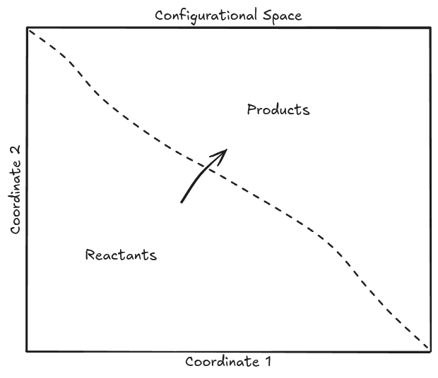
Figure 1: Arbitrary atomic configuration map with regions separated into reactants and products via a dividing surface (dashed line). Reactions happen when the configuration of atoms traverses the dividing surface and goes from the region of reactants to products (and back for reversible reactions).
The most straightforward way to simulate this (if we assume no quantum tunneling and only one, elementary reaction) would be to use ab initio molecular dynamics to model the system and count every time the system traverses the dividing surface from reactants to products. This mirrors how reactions happen in the "real world," but is prohibitively expensive for all but the simplest systems. Atoms are constantly bouncing around, but only rarely do they react—the energy barriers are large and the reaction channel the atoms need to funnel through is very narrow (thus giving rise to enthalpic and entropic penalties to reaction).
Instead of modeling the dynamics explicitly, if we assume that the reaction only occurs in one direction (i.e. this is not a reversible reaction), we can predict the rate of the reaction from the thermal energy in the system and the difference between the energy of the reactants and the energy on the dividing surface (we call this the "barrier energy" and need to use a partition function to model the energy of the atoms in the reactant space and the energy of the barrier separating the reactant space from the products).
To illustrate, if we take the toy system of linear H + H₂ we can see the energy landscape as we change the interatomic distances separating the hydrogen atoms. Most of the potential energy surface (PES) is much too high in energy for the atoms to ever reach. Instead they are confined to a narrow, curving channel of probable reaction configurations.
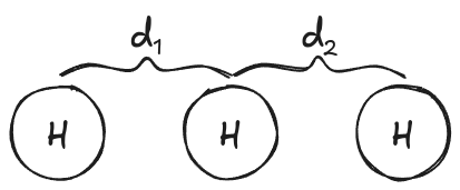
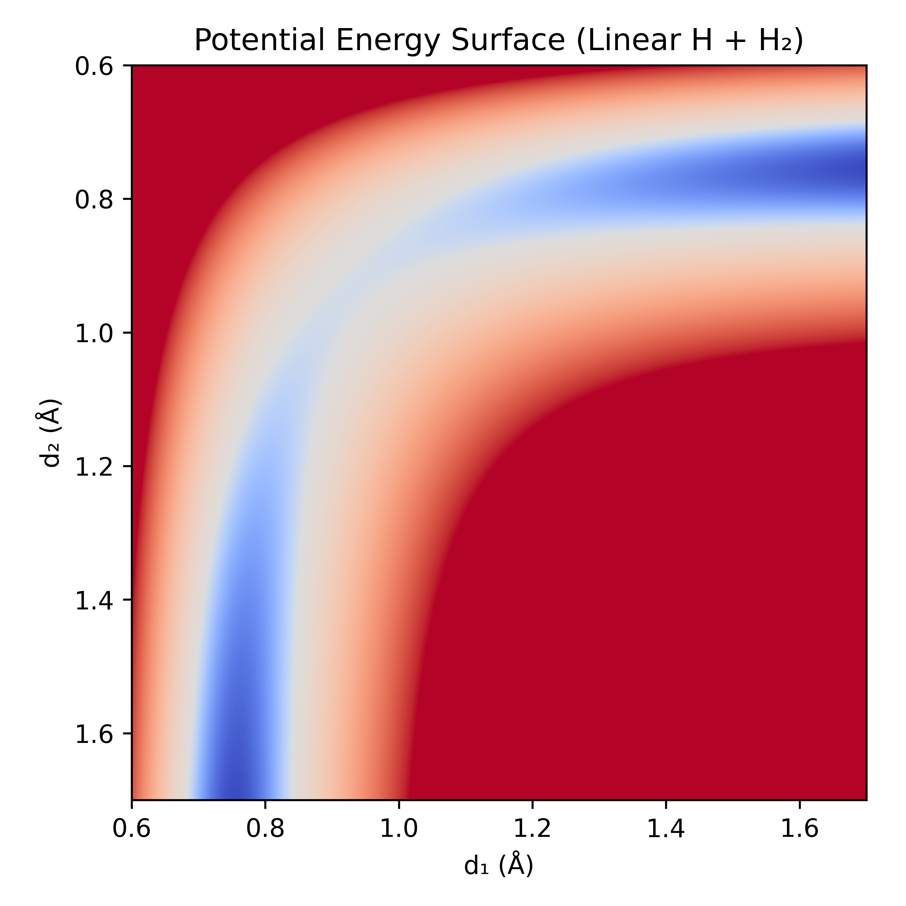
Figure 2: Linear H + H₂ potential energy surface (PES) calculated with r²SCAN-3c. Blue indicates low-energy, red indicates high-energy. Note: the color map is non-linear to better see what is happening at the bottom of the well.
We can draw a separating surface along the ridge line between these two regions (illustrated here with the diagonal dashed black line) and compare its energy to the energy of the reactant region.
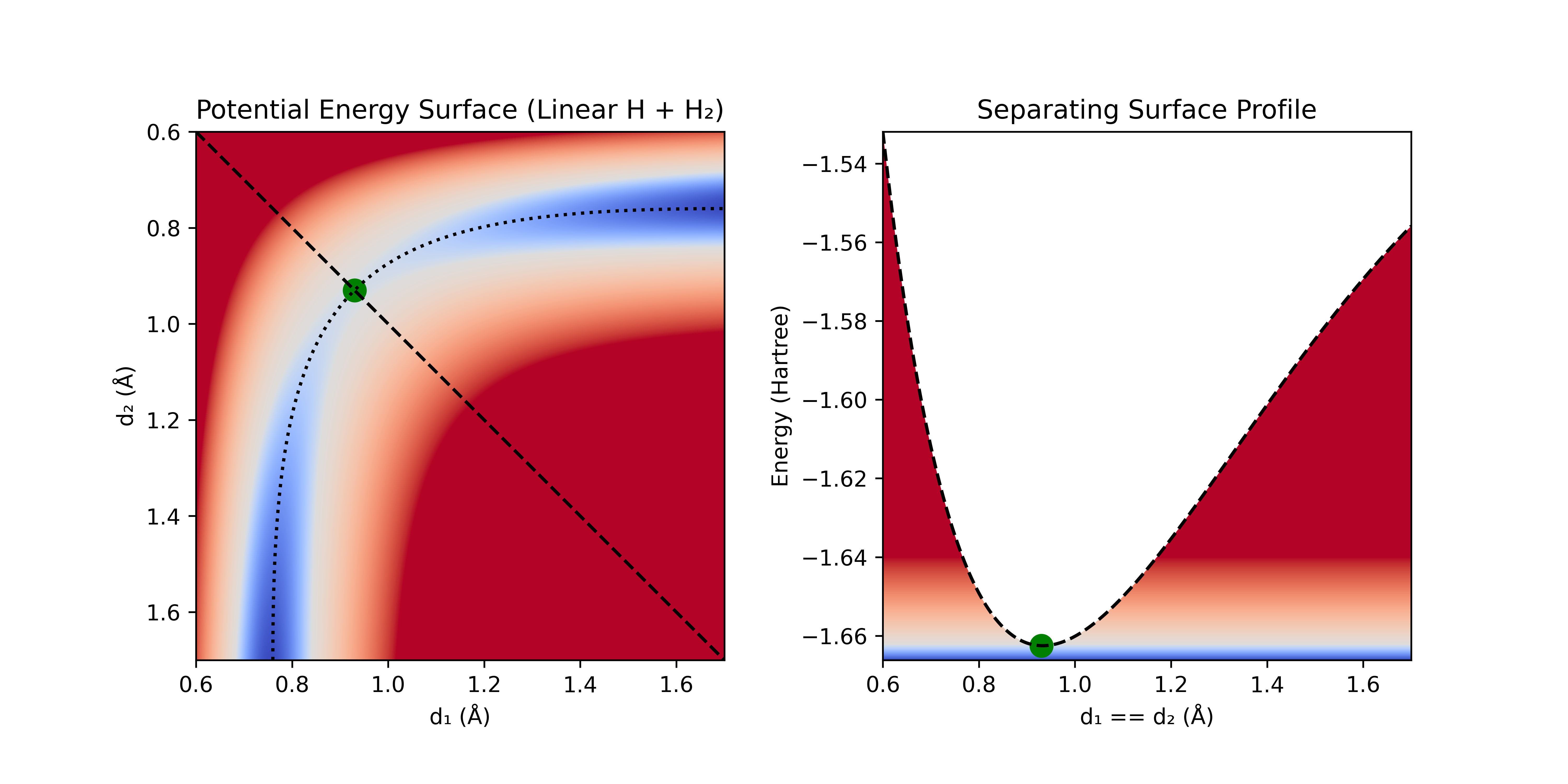
Figure 3: A) Linear H + H₂ PES with dividing surface (black dashed line), IRC (dotted black line), and TS (green dot). B) Energy along dividing surface (dark blue line represents the minimum energy of the system).
For more complicated systems, the dividing surface is an ()-dimensional hyperplane separating the two regions, and determining it precisely is prohibitively expensive for all but the simplest systems.
For low-energy systems (e.g. <1000 K), most of the flux between reactants and products will occur through the narrow region of space where the barrier is the lowest. This is similar to how most traffic between regions separated by mountain ranges happens through mountain passes—the lowest point along the ridge line. Instead of calculating the flux through the entire dividing surface, we can compute it only for the low energy regions and presume it is 0 everywhere else. We can make a further simplification, and use the lowest energy point along this dividing surface as a proxy for the whole ridge line (if we assume that there are no other low-lying points).
This lowest energy point on the dividing surface is termed the transition state (TS), and is often likened to a horse saddle or a pringle (mathematically, it is referred to as a 1st-order saddle point). It has negative curvature along one coordinate (the coordinate corresponding to the reaction), and positive curvature along all other coordinates. It has the interesting property of also being the highest energy point along the lowest-energy path connecting reactants and products (assuming an elementary reaction). Since precisely determining the partition function between the reactant and product regions is non-obvious, and finding the lowest energy point along this partition is incredibly difficult, we can instead solve the simpler (but far from easy problem) of determining the highest energy point along the lowest-energy path connecting the reactants and products.
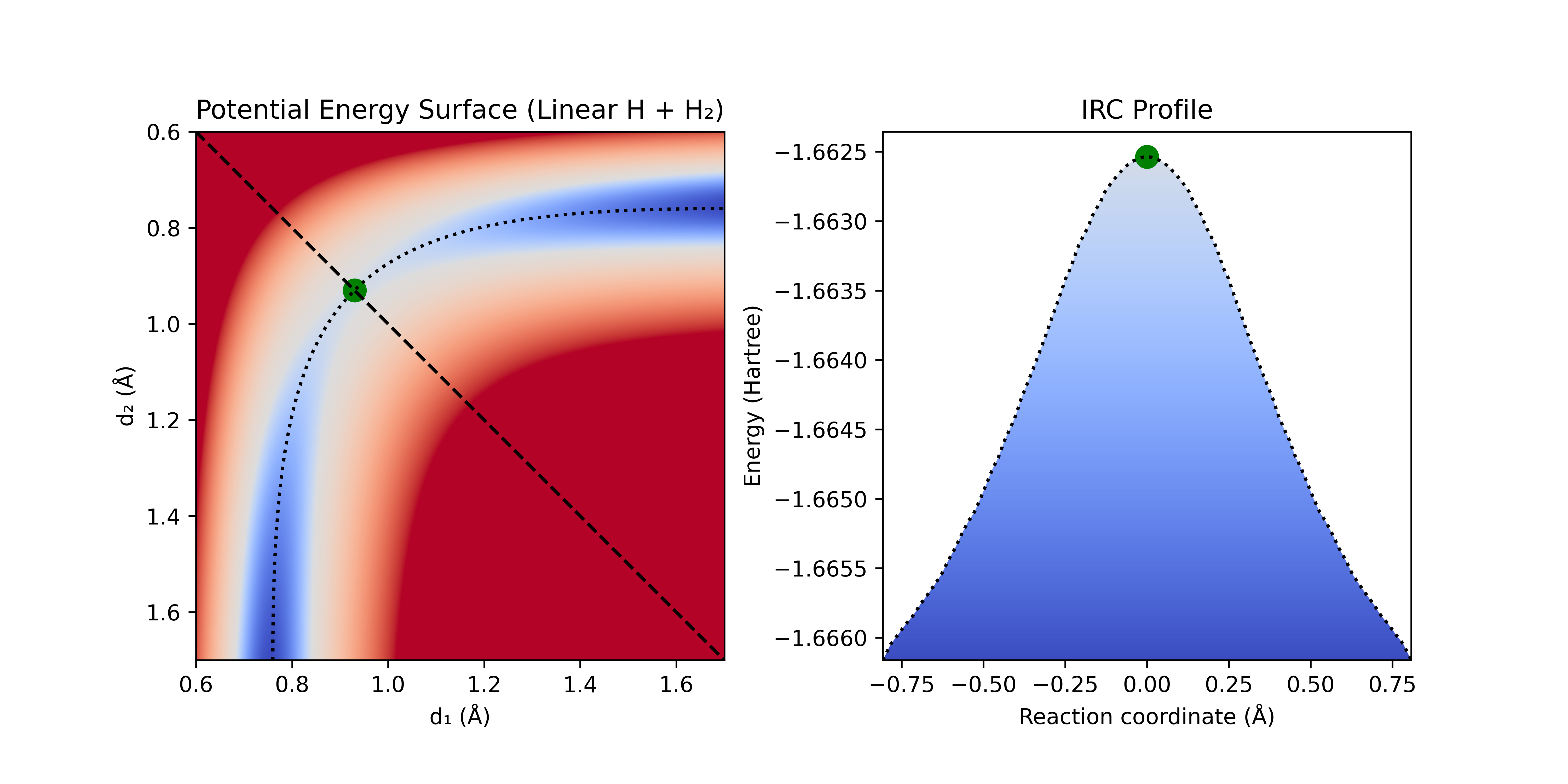
Figure 4: Linear H + H₂ PES and the intrinsic reaction coordinate (IRC) connecting reactants and products. Note the difference in energy scale for the IRC profile from the separating surface in figure 3.
We can see that the transition state for H + H₂ has a gradient of zero in all directions, and curvature that is negative along the IRC and positive orthogonal to the IRC. Finding this transition state is relatively simple for this system, but for larger systems it can become incredibly complicated.
Transition State (TS) Optimization
There are many approximate methods to generate a guess for transition states that are beyond the scope of this article (see Corin's video on finding transition states). Once a guess has been generated, it can be optimized to the true transition state. Approximate second-order methods are typically used, where the Hessian (matrix of mixed second derivatives showing the curvature at a point) is calculated and then diagonalized to find the curvature of the surface. Positive eigenvalues indicate positive curvature in the direction of their corresponding eigenvector, while negative eigenvalues indicate negative curvature in the direction of the corresponding eigenvector. The frequency is proportional to the square root of the eigenvalue, and thus imaginary frequencies indicate negative curvature (imaginary frequencies are often simply reported as negative).
Once the eigenvector corresponding to the reaction is identified (typically the one with the most negative eigenvalue, but sometimes one containing certain molecular motions), an optimization is performed where steps are taken along the target coordinate in the direction that maximizes its energy while simultaneously minimizing the energy along all of the other coordinates. Once the gradient is zero in all directions and there is only one negative eigenvector, a saddle point has been reached.
Intrinsic Reaction Coordinate (IRC)
To confirm that the saddle point is a transition state connecting reactants and products, it is necessary to calculate the intrinsic reaction coordinate (IRC). An IRC calculation follows the forward and backwards paths of steepest descent down the potential energy surface from the transition state toward both reactants and products (analogous to the fall line in topography). It takes a fixed step sizes (in mass-weighted coordinates) along the forward and backward directions of the reaction coordinate until it hits its target number of steps, or a minimum has been found.
IRC calculations can be divided into two categories: explicit and implicit. Explicit methods use only the data at the current position (e.g. gradient and approximate Hessian) to chose the next step (e.g. second-order Newton methods with a fixed step size). Implicit methods use the data at the current position, and information about the gradient at a pivot point some distance from the starting point to find the the optimal next step. Explicit methods are prone to drifting off the IRC when sharp turns are encountered, and often require very small step sizes. Implicit methods can take significantly larger steps, as they approximate the accuracy of fourth-order methods.
This process of taking steps is repeated until it has been determined that the reactants and products are connected—typically with a fixed number of steps or a set convergence criteria. This can be further augmented by performing an optimization starting from the final step in each direction of the IRC to obtain the true minima in the reactant and product regions. Due to the fixed step size, the IRC cannot land directly on the true minimum, and for reactions that start or end with dissociated molecules, it would be ill-advised to run them to infinity.
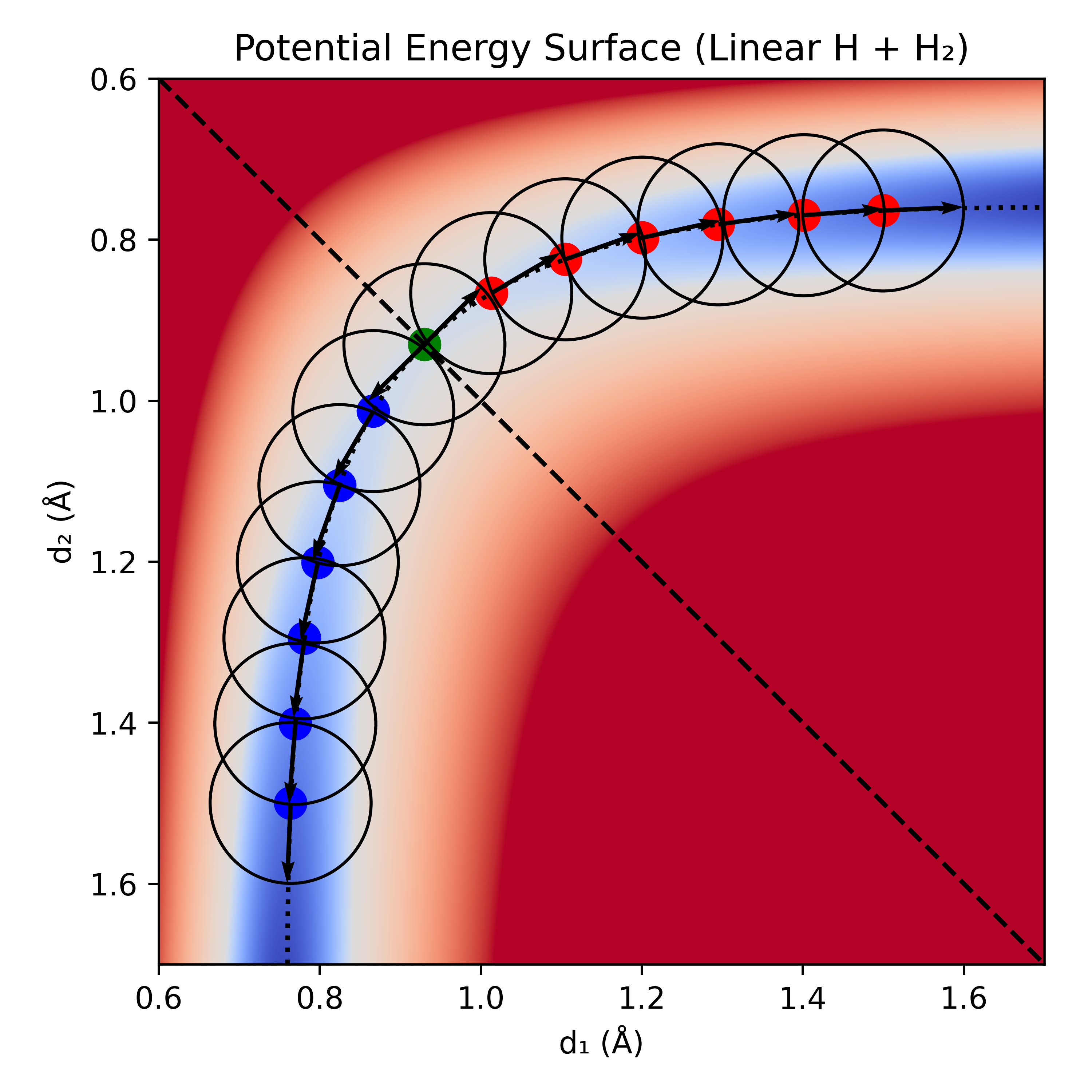
Figure 5: IRC with 6 steps in each direction and a fixed step size of . The direction of the gradient/coordinate at each step is indicated with an arrow; naïvely following it would cause a calculation to stray from the true IRC, thus showing the need for higher-order methods.
There are many tricks for improved transition state optimization and IRC optimization that are beyond the scope of this article, such as improved coordinate representations (e.g. geomeTRIC) and updating of the Hessian with a subset of second derivatives. Most programs calculate an exact Hessian at the beginning of the calculation and approximately update it every step. Once a set number of steps have been taken, the exact Hessian is recalculated, and this process is repeated until convergence has been reached. Due to the difficult nature of these optimizations, it is often necessary to set tighter convergence criteria, and not uncommon for them to fail by wandering off in the wrong direction, and more work is needed in this area to help increase the robustness of common algorithms.
To model your own reactions with these techniques, you can use Rowan's quantum chemistry web platform. Rowan's reaction modeling toolkit currently includes:
- scans (very useful for finding guess transition states),
- transition-state optimizations,
- transition-state conformer searches, and
- intrinsic reaction coordinates (IRC).
If you want to learn about how to generate better initial starting geometries for transition state optimization, check out our blog on guessing transition states. You can also create a free account and start modeling reactions in minutes!