How to Predict Protein–Ligand Binding Affinity
by Corin Wagen · Feb 11, 2026
Prediction of protein–ligand binding affinity is one of the most common and crucial tasks in computer-assisted drug design. Despite the multiparametric nature of drug discovery, achieving good binding affinity remains central to the development of a successful therapeutic: a recent perspective by Mark Murcko argues that the importance of optimizing binding affinity remains underrated.
Unfortunately, accurate computational prediction of binding affinity is extremely difficult. Binding affinity depends not only on the static structures of protein–ligand complexes, which are themselves difficult to predict with experimental accuracy, but also on a host of even more complex and difficult-to-predict factors: subtle non-covalent interactions between ligand atoms and protein sidechains, the structure and behavior of the water solvation shell, the conformational motion of protein and ligand, and the interplay between entropy and enthalpy in determining the ultimate free energy of binding.
Since ideal solutions to these problems are usually prohibitively expensive (if not outright impossible), practical binding-affinity prediction relies on a large number of bespoke approximations which can be deployed at various points in a project lifecycle. This post aims to (1) give a high-level overview of seven widely used approaches in practice, (2) briefly explain how each approach works (and where it might fail), and (3) help novice drug designers choose the right tool for the right occasion in a program.
(Before we start, a necessary disclaimer: this is an exceptionally large and complex field, and the present post does not aspire to be an exhaustive review. Rather, this is intended to be a high-level overview for newcomers to the field. Experienced practitioners will no doubt take issue with some of the statements here; although we've tried to be correct and minimally misleading, inaccuracies certainly remain.)
What do we mean by binding affinity?
Experimentally, teams often work with several related readouts, including Kd and Ki, and assay-dependent quantities like IC50. Kinetic parameters that imply residence time (kon, koff) are also sometimes used. Most physics-based methods aim to estimate a binding free energy, ΔGbind, because it connects most directly to thermodynamic definitions of binding. With appropriate assumptions about the binding model and assay conditions, ΔGbind can be related to Kd or Ki. Unlike Kd or Ki, IC50 is assay- and mechanism-dependent, and it only maps to an inhibition constant under additional assumptions (for example, via the Cheng–Prusoff relationship for simple competitive inhibition)
It is worth noting that even "gold-standard" experimental measurements carry nontrivial uncertainty. Across labs and assay formats, reported Kd and Ki values for the same system can differ by a few tenths of a log unit, and sometimes more. This variability is an important reality check for any model trained on heterogeneous public data, though tighter floors are possible in a single well-controlled assay.
Lower-cost methods often produce uncalibrated scores that are used primarily for ranking rather than for absolute ΔG prediction. Docking scores are best treated as heuristic ranking signals, and even methods that output "ΔG-like" values with energy units (such as MM/GBSA) are usually used for relative ranking unless carefully calibrated.
In practice, many teams layer methods together: docking to generate poses, MM/GBSA or ML rescoring to refine ranking, and FEP on a focused set of top candidates. Most of the individual methods below can be (and often are) used in combination, and a layered workflow is often more effective than relying on any single approach.
1. Ligand-based similarity methods
Ligand-based virtual screening starts from the heuristic that similar molecules often have similar activity, while recognizing that activity cliffs are common. The simplest and most ubiquitous operationalization of this is 2D fingerprint similarity—computing Tanimoto coefficients over extended-connectivity fingerprints (ECFP4/Morgan fingerprints) to identify analogs of known actives. This is fast, trivially parallelizable, and often a surprisingly strong baseline.
Shape-based methods extend similarity into 3D by aligning molecules and scoring how well their volumes and pharmacophoric features overlap. ROCS (Rapid Overlay of Chemical Structures) is the classic example; FastROCS is the high-throughput GPU-accelerated version designed for very large libraries. The "color" component of ROCS, which captures overlap of pharmacophoric and chemical features beyond simple 3D shape, is often critical; shape alone can miss many meaningful chemical distinctions (e.g. pyridine vs benzene).
Pharmacophore models are a related ligand-based approach. Rather than comparing full molecular shapes, pharmacophore methods define an abstract spatial arrangement of chemical features (hydrogen-bond donors & acceptors, hydrophobic regions, aromatic rings, charged groups, and so on) and screen for molecules that match. Pharmacophore models can be built from a set of known actives alone or combined with protein-structure information; they are particularly useful for scaffold hopping, since chemically dissimilar molecules can satisfy the same feature geometry.
When you have a known ligand and you care about finding analogs or scaffold hops that preserve key features, similarity and pharmacophore methods can be extremely cost-effective. A key limitation is the need for at least one reasonable query ligand (and, for 3D methods, a plausible query pose), and performance can degrade when the binding mode is not conserved or when active structures are diverse in shape.
Key publications:
- Rogers and Hahn, J. Chem. Inf. Model. 2010—Extended-Connectivity Fingerprints (ECFP), the most widely used fingerprint family in pharmaceutical research
- Grant, Gallardo, and Pickup, J. Comput. Chem. 1996—the Gaussian shape overlay concept underlying ROCS
- Rush et al., J. Med. Chem. 2005—prospective validation of shape-based virtual screening
- Hawkins et al., J. Med. Chem. 2007—direct comparisons of shape-based methods vs. docking in screening benchmarks
Representative tools:
- OpenEye ROCS/FastROCS (shape)
- RDKit (fingerprints, pharmacophores)
- Schrödinger Phase (pharmacophore + shape)
2. Docking and classical scoring functions
Docking tries to answer two questions: (1) what pose does the ligand adopt, and (2) how good is that pose? Most docking engines generate many poses in a binding site and rank them with a scoring function that mixes simplified physics with empirical calibration. Docking is fast enough for screening, provides interpretable poses, and is often the first structure-based method that drug-discovery teams reach for.
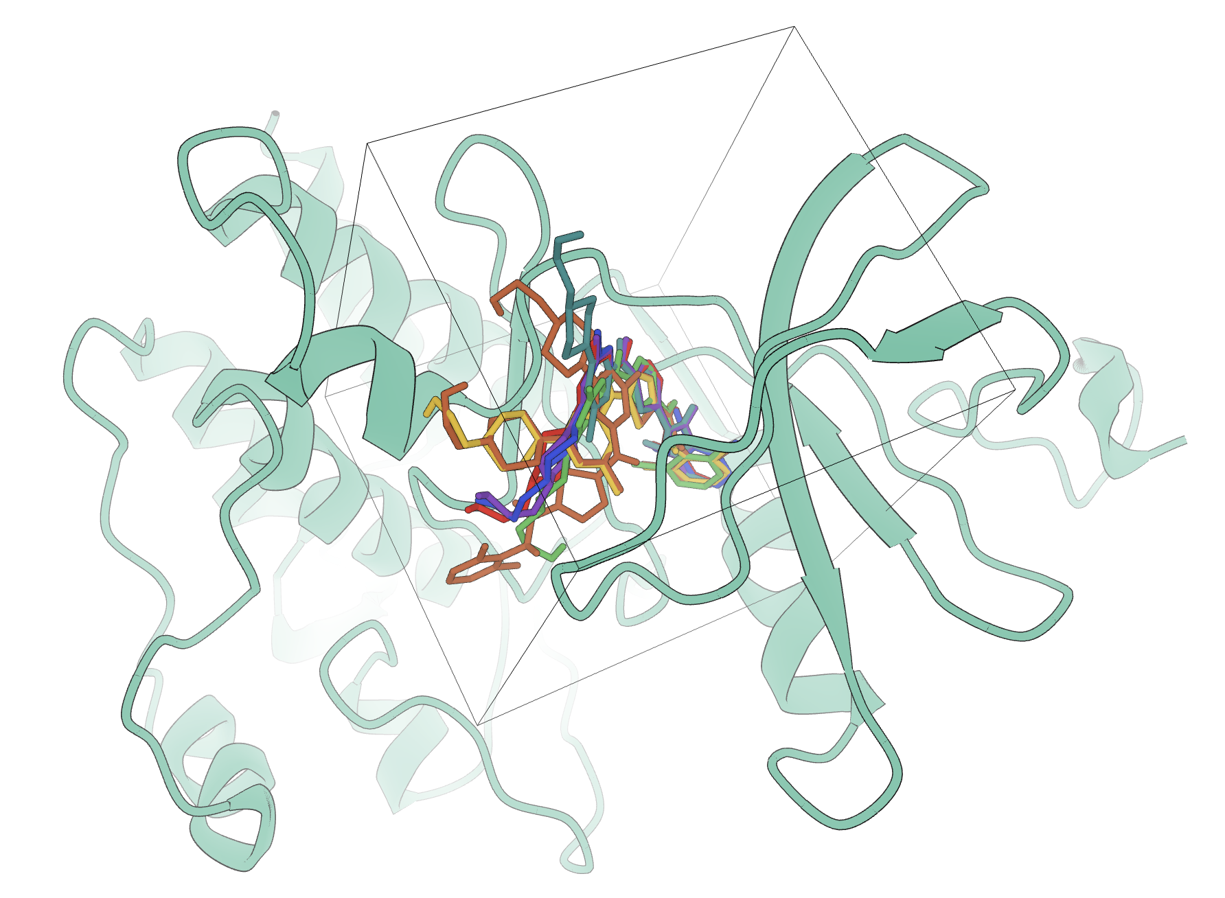
A visual representation of different docking poses bound to the protein target. The pocket for docking is visible as a cube.
In practice, docking scores are usually poor surrogates for binding free energies, especially across diverse chemotypes. Scoring functions fail to account for numerous physical effects: protein flexibility, waters and ions, alternate protonation states, strain and desolvation effects, and more. As a result, docking is often more reliable for pose generation than for potency ranking, particularly when protein flexibility, waters, or protonation states matter, and obtaining meaningful enrichment from docking scores at scale requires considerable caution. Benchmarking docking enrichment is itself non-trivial—the DUD-E benchmark set (Mysinger et al., 2012) is widely used but has known biases that can inflate apparent performance, particularly for machine-learned models.
Some of these limitations are manageable in practice. Water thermodynamics analyses can help identify conserved and displaceable waters and can sometimes improve pose selection and triage, though results are system- and protocol-dependent. Similarly, careful attention to protonation and tautomeric states, supported by tools that enumerate relevant forms for both protein and ligand, can help.
Key publications:
- Friesner et al., J. Med. Chem. 2004—Glide, probably the most widely used docking program in pharmaceutical research
- Jones et al., J. Mol. Biol. 1997—GOLD, genetic-algorithm-based docking
- Trott and Olson, J. Comput. Chem. 2010—AutoDock Vina, a widely used open-source docking engine
- Yu et al., J. Chem. Theory Comput. 2023—Uni-Dock, GPU-accelerated Vina for ultra-large-scale docking
- Mysinger et al., J. Med. Chem. 2012—DUD-E, the standard benchmarking set for docking enrichment
Representative tools:
- Schrödinger Glide
- GOLD (CCDC)
- AutoDock Vina
- FRED (OpenEye)
- rDock
3. QSAR and supervised ML potency models
Quantitative structure–activity relationship (QSAR) models learn relationships between chemical structure and activity from experimental data. These can range from simple linear models on hand-crafted descriptors to modern deep-learning approaches including graph neural networks, transformers, and multitask models. If you have a consistent assay and enough data within a chemical series, QSAR is often the fastest way to get useful potency prioritization.
At the simplest end, Free–Wilson analysis (Free and Wilson, 1964) decomposes activity into additive contributions from substituents at defined positions on a shared scaffold. This remains a valuable tool in lead optimization: it is interpretable, fast to build, and can perform well when additivity approximately holds. (Pat Walters has demonstrated a Python implementation of Free–Wilson analysis on his Practical Cheminformatics blog.)
Matched molecular pair (MMP) analysis is a related idea—rather than decomposing activity on a scaffold, MMP analysis identifies pairs of molecules that differ by a single structural transformation and tabulates the associated activity change. MMP databases built from large corporate datasets can be remarkably useful for predicting the effect of common medicinal chemistry moves.
Modern ML-based QSAR typically uses molecular graph- or fingerprint-based representations fed to random forests, gradient-boosted trees, or graph neural networks. These approaches can capture nonlinear SAR and generalize further than Free–Wilson analyses, but they can also struggle in practice: a model can look excellent under retrospective random splits yet fail prospectively when the next design cycle moves into new chemical space or changes assay context. Understanding when and how QSAR models fail—and designing evaluation protocols (temporal splits, scaffold splits) that expose these failures before they matter—is at least as important as choosing the right architecture.
Key publications :
- Free and Wilson, J. Med. Chem. 1964—additive group contribution model for congeneric SAR
- Griffen et al., J. Med. Chem. 2011—matched molecular-pair analysis applied to large pharma datasets
- Svetnik et al., J. Chem. Inf. Comput. Sci. 2003—random forests for QSAR, still a strong baseline
- Yang et al., J. Chem. Inf. Model. 2019—Chemprop, directed message-passing neural networks for molecular property prediction
- Wallach and Heifets, J. Chem. Inf. Model. 2018—"Most Ligand-Based Classification Benchmarks Reward Memorization Rather than Generalization," an important critique of ML scoring evaluation
Representative Tools:
- Chemprop
- RDKit + scikit-learn
- Schrödinger AutoQSAR
4. Endpoint free-energy methods: MM/GBSA, MM/PBSA, and related approaches
MM/GBSA and MM/PBSA compute a ΔG-like score by combining molecular-mechanics terms with an implicit-solvent model (and optionally an approximate entropy term), typically over MD snapshots. They are often called "endpoint" methods because they do not explicitly alchemically transform one ligand into another, instead comparing bound and unbound states for a given ligand.
In practice, these endpoint methods occupy a middle ground between docking and full free-energy methods. They are often more physically motivated than docking scores and can incorporate local relaxation, but they remain highly protocol-sensitive: implicit solvent is an aggressive approximation, conformational sampling is typically limited, and entropy estimation is imperfect and protocol-dependent. They can be useful for pose rescoring and for rough comparisons within closely related sets, but prospective performance varies widely with force field, sampling, and solvation-model choices.
(Read about our efforts to build next-generation endpoint methods with machine learning here!)
Linear interaction energy (LIE) is a related endpoint approach that estimates binding free energy from the average electrostatic and van der Waals interaction energies between ligand and surroundings in bound and free states, scaled by fitted coefficients. LIE is conceptually simpler than MM/GBSA and avoids some of its approximations (particularly the implicit-solvent decomposition), but requires empirical parameterization and has seen less widespread adoption.
Semiempirical quantum chemistry has also been explored as a single-structure or limited-sampling scoring approach. SQM2.20 uses a semiempirical QM Hamiltonian to score protein–ligand complexes directly; the authors have reported strong benchmark performance and external evaluations are starting to appear, but its practical domain of reliability is still being mapped.
Key publications:
- Genheden and Ryde, Expert Opin. Drug Discov. 2015—review of MM/PBSA and MM/GBSA for ligand binding
- Åqvist et al., Protein Eng. 1994—linear-interaction-energy method
- Rifai et al., Nat. Commun. 2024—semiempirical QM scoring of protein–ligand complexes
- Sindt et al., J. Chem. Inf. Model. 2025—comparison of different docking rescoring methods
Representative tools:
- AMBER MMPBSA.py
- Schrödinger Prime MM-GBSA
- gmx_MMPBSA (GROMACS)
- xTB
5. Relative binding free-energy perturbation (RBFE FEP)
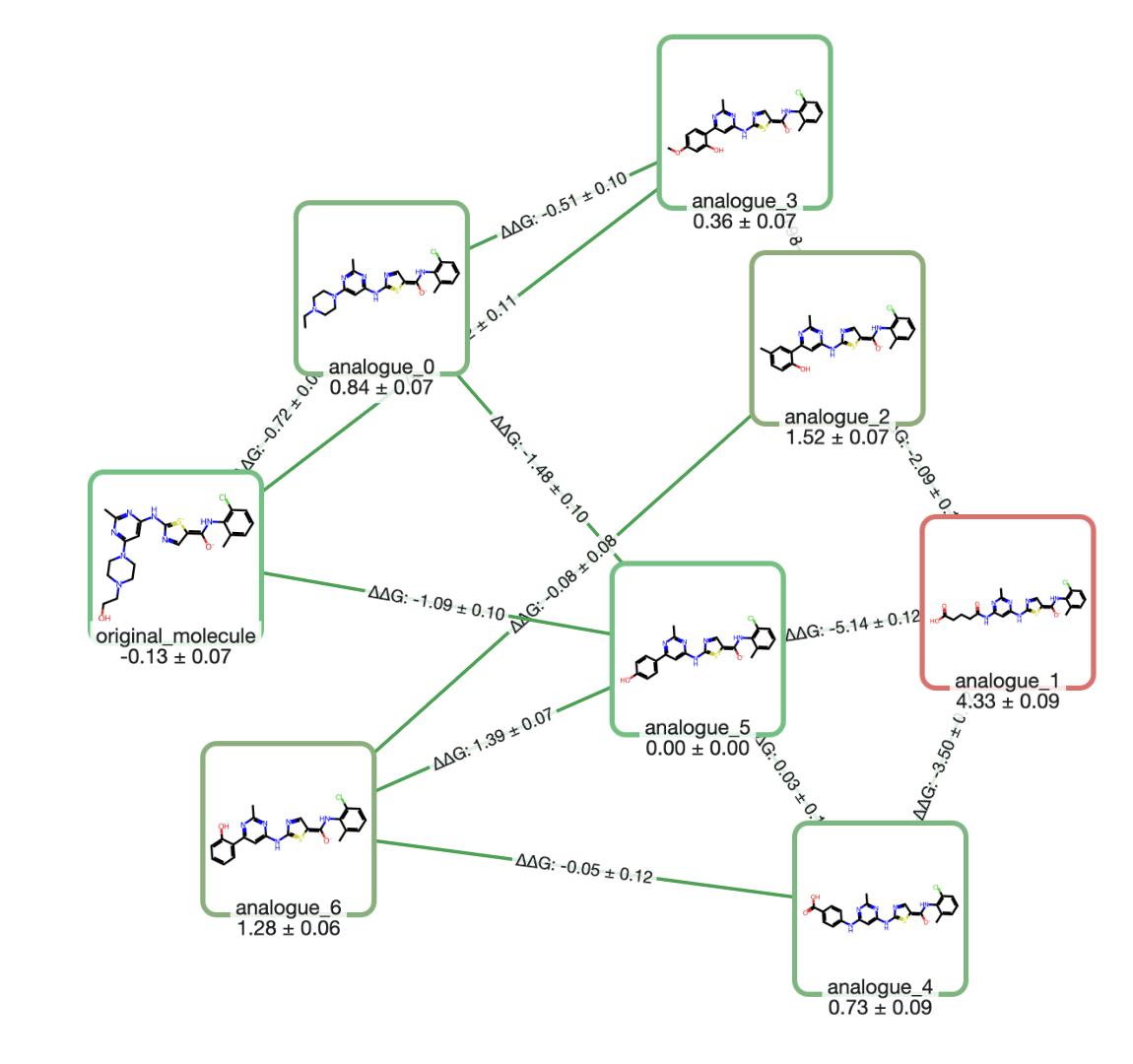
Relative binding free-energy methods compute the change in binding free energy between two ligands by "alchemically" transforming one ligand into another in both solvent and the protein complex. The output is ΔΔG between ligands, which is often exactly what a medicinal chemist needs for SAR ranking. Because many systematic errors partially cancel between similar ligands, RBFE can be among the most accurate prospective options for congeneric series when binding modes are stable. (Read more about what FEP requires on our dedicated FEP page.)
The main practical constraints are setup complexity, sampling, and overall cost. Robust RBFE requires sensible ligand mappings, careful handling of protonation and tautomers, attention to net charge changes, and enough sampling to converge relevant degrees of freedom. Conversely, RBFE can struggle when ligands change binding mode, when slow protein motions matter, or when the water network reorganizes substantially across the series.These failure modes are increasingly addressable: REST2 (replica exchange with solute tempering) & related enhanced-sampling techniques can improve convergence for slow degrees of freedom and grand canonical methods for water insertion & deletion can handle cases where the water network changes between ligands.
An example of a sample output graph from an RBFE FEP calculation.
Computational cost remains considerable, however. RBFE calculations, while faster than absolute binding free-energy calculations (vide supra), are still pretty slow compared to other computational chemistry methods. In production-like protocols, RBFE commonly costs on the order of single to tens of GPU-hours per edge, depending on sampling, repeats, and the difficulty of the transformation. In cloud settings, marginal compute costs per evaluated edge can be nontrivial ($10 or more), which is why most teams reserve RBFE for a focused set of high-value decisions.
Development of improved RBFE engines remains an important scientific area. Various companies and research groups are investigating the use of neural network potentials or low-cost quantum-chemical methods as more accurate replacements for force fields, while other teams are studying ways to accelerate RBFE calculations through techniques like local resampling and non-equilibrium switching.
Key publications:
- Wang et al., J. Am. Chem. Soc. 2015—the landmark FEP+ paper demonstrating practical industrial usage
- Gapsys et al., Chem. Sci. 2020—non-equilibrium free energy calculations with pmx/GROMACS
- Loeffler et al., J. Chem. Theory Comput. 2018—investigation of the reproducibility of RBFE calculations
- Mey et al., Living J. Comp. Mol. Sci. 2020—best practices for alchemical free energy calculations
- Schindler et al., J. Chem. Inf. Model. 2020—large-scale benchmarking of industrial RBFE
Representative tools:
- Schrödinger FEP+
- OpenFE
- pmx (GROMACS-based)
- NAMD FEP
6. Absolute binding free-energy perturbation (ABFE FEP)
Absolute binding free energy methods aim to compute ΔGbind for a single ligand, typically by applying restraints and alchemically decoupling the ligand from its environment. ABFE is appealing because it promises transferability across chemotypes, including cases where there is no obvious mapping between ligands.
In practice, ABFE is harder to converge than RBFE. Convergence is more challenging—ABFE typically requires substantially more sampling per compound than RBFE, which translates into slower and more expensive calculations—and results are more sensitive to protocol choices. Waters, multiple binding modes, and protein reorganization can dominate the error budget, and they are hard to capture reliably without substantial sampling. That said, there has been significant progress, and ABFE is increasingly used in targeted scenarios where RBFE is not applicable: comparing hits from different chemical series, evaluating fragment binding hypotheses, or connecting distinct scaffolds within a program.
Key publications:
- Gapsys et al., Commun. Chem. 2021—demonstration of accurate ABFE with equilibrium and non-equilibrium approaches
- Mey et al., Living J. Comp. Mol. Sci. 2020—best practices discussion including ABFE
Representative tools:
- AMBER
- GROMACS (with pmx)
- OpenMM
- NAMD
- OpenFE
7. Structure-based ML scoring
A newer category of methods predicts potency-like values or ranking scores from a 3D protein–ligand complex using machine learning. These range from models that score a given pose (analogous to a classical scoring function, but learned from data) to models that jointly predict the 3D structure and affinity from sequence and SMILES alone. The distinction matters because pose-conditioned models inherit pose errors, while joint structure-plus-affinity models compound uncertainty from two difficult predictions.
Among pose-scoring models, early examples include RF-Score (Ballester and Mitchell, 2010), which applied random forests to interaction features, and more recent neural approaches like KDEEP (Jiménez et al., 2018) and gnina (McNutt et al., 2021), which use convolutional neural networks on voxelized representations of the binding site. AEV-PLIG is another representative example, producing affinity estimates from bound complex structures quickly enough for interactive use.
On the joint-prediction side, Boltz-2 (Wohlwend et al., 2025) predicts both the 3D structure of the protein–ligand complex and a binding affinity estimate starting from protein sequence and ligand SMILES. (For more details, see our Boltz-2 FAQ.) DiffDock (Corso et al., 2023) uses a diffusion generative model for pose prediction with learned confidence scores, though it does not directly predict affinity.
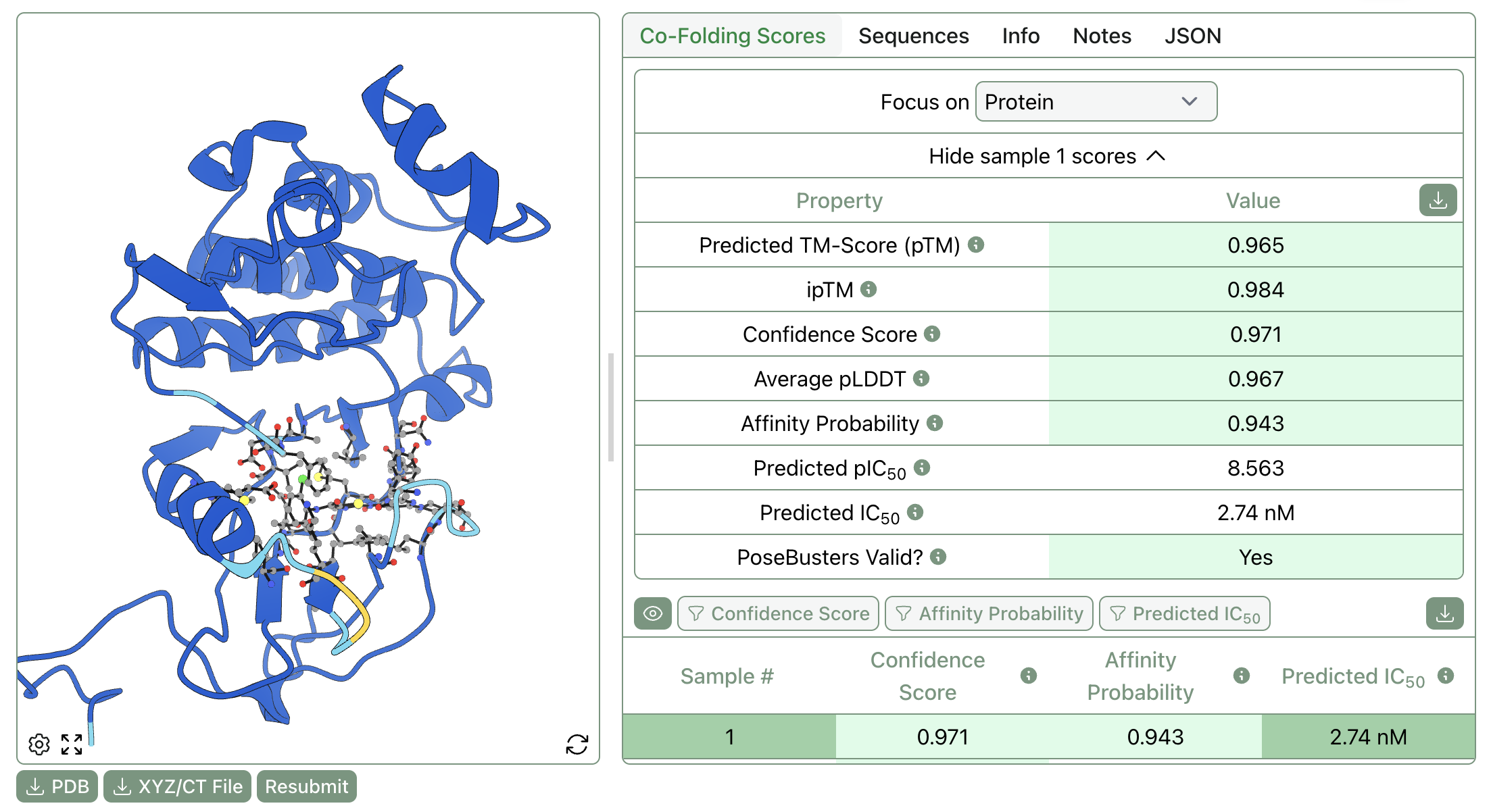
An example of a Boltz-2 calculation with associated binding-affinity predictions.
Many structure-based ML scoring functions perform best near their training distribution and can degrade on new targets, new protein families, or novel chemotypes. A growing body of work has focused on understanding and mitigating this problem. Much of the field has historically trained on PDBbind (Wang et al., 2004), which has well-documented biases: random train/test splits leak information through protein family and ligand similarity, and temporal or scaffold-based splits reveal substantially worse generalization. Careful evaluation hygiene—using time-based splits, target-based splits, or prospective validation—is essential for understanding what these models can actually do.
A practical way to think about these models is as learned scoring functions that can be extremely useful within a validated domain, but that should not be assumed to generalize without targeted testing. They can be very useful for triage and ranking when you have plausible poses, but they should be validated in the specific context you plan to use them, especially when making expensive synthesis decisions.
Key publications:
- Ballester and Mitchell, Bioinformatics 2010—RF-Score, an early and influential ML scoring function
- Jiménez et al., J. Chem. Inf. Model. 2018—KDEEP, CNN-based scoring
- McNutt et al., J. Cheminf. 2021—gnina, CNN scoring integrated with docking
- Wang et al., J. Med. Chem. 2004—PDBbind, the primary training and benchmark dataset for much structure-based ML scoring
- Su et al., J. Chem. Inf. Model. 2020—analysis of train–test similarity in PDBbind
- Corso et al., ICLR 2023—DiffDock, diffusion-based blind docking
- Wohlwend et al., 2025—Boltz-2, joint structure and affinity prediction
Representative tools:
- gnina
- Boltz-2 (open-source) and Boltz-2.1 (closed-source; Boltz-hosted)
- DiffDock
- AEV-PLIG
Which approach should you use?
No single method is best across all stages of a program, but a method's cost and failure modes can be matched to the decision at hand.
If you are doing hit finding or exploring ultra-large libraries, prioritize throughput and enrichment. Ligand-based similarity methods (fingerprints, shape, pharmacophores) and docking are often the right first layer, sometimes combined with fast ML rescoring when you have plausible poses.
If you are in lead optimization with a congeneric series and stable binding mode, RBFE FEP is usually the most decision-relevant tool because it targets ΔΔG directly and tends to be most accurate when chemical changes are incremental. For simpler SAR questions in a well-behaved series, Free–Wilson or MMP analysis may give you what you need faster.
If you need to compare across scaffolds, ABFE and carefully validated structure-based ML models become more attractive, but you should expect higher variance and more protocol sensitivity than in RBFE.