Exploring Protein–Ligand Binding-Affinity Prediction
by Ishaan Ganti · Aug 20, 2025
Corin here! I had the pleasure of supervising Ishaan this summer. While we didn't end up finding a fast and accurate protein–ligand rescoring method like we hoped to, Ishaan did fantastic work. He was able to quickly try out a wide array of different physics- and ML-based approaches and make critical decisions in a rigorous and data-driven way.
We wanted to share what we learned so that future teams can benefit from Ishaan's hard work—and we hope to ship something in this area in the future. I'll let Ishaan take it from here.
This summer, I worked at Rowan on building better "medium-compute" binding-affinity-prediction techniques. While I wasn't successful at directly achieving this goal, I came away with a few insights I think are worth sharing.
In drug discovery, "binding affinity" refers to the strength with which a small molecule (ligand) binds to a target protein/gene. Candidate drugs must, before all else, bind strongly to the target site—otherwise, they can't be effective. To grasp how effective these tools are, some important things to keep in mind:
- Binding affinities are essentially always in the −20 kcal/mol to 0 kcal/mol range. Most are in the −15 kcal/mol to −4 kcal/mol range.
- Binding affinity is a free energy; more negative values indicate a more thermodynamically favorable process.
- Standard drug-discovery settings prioritize relative rankings more than absolute numerical agreement with experimental binding affinities. So, even if my predicted binding affinities are incorrect, they can be useful.
Today's binding-affinity-prediction tools span a large area on the speed–accuracy plane.
At one end is docking, which offers fast but extremely inaccurate results. For some rough figures, docking generally takes less than a minute on CPU and delivers results with 2–4 kcal/mol RMSE. Correlation coefficient values vary significantly based on system, but I've seen values around 0.3 most frequently.
At the other end we have techniques like free energy perturbation (FEP) and thermodynamic integration (TI), which make use of extensive molecular dynamics (MD) simulation to achieve impressive accuracy. However, the 12+ hours of GPU time required for this class of approaches renders them impractical for tens of thousands of candidates. Correlation coefficients of 0.65+ can be expected here, and RMSE values tend to hover around just below 1 kcal/mol.
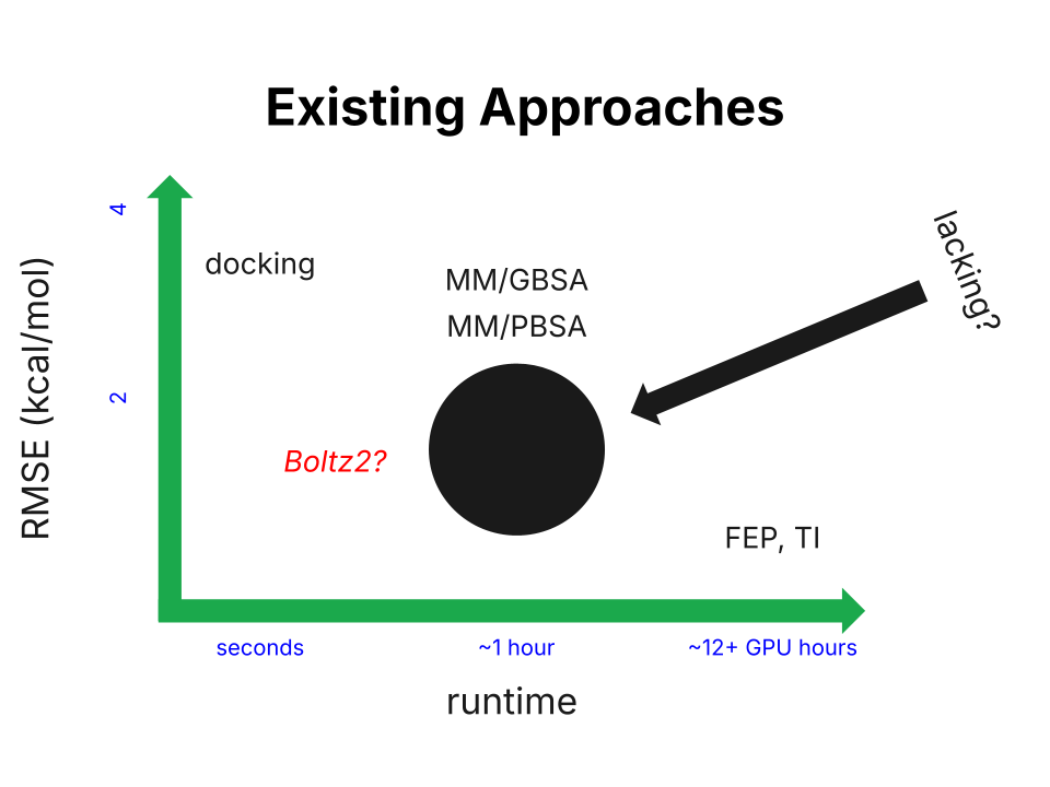
Existing approaches to protein–ligand binding-affinity prediction, roughly compared.
There's a clear methods gap here; the space yearns for something definitively more accurate than docking but faster than FEP. The MM/PBSA and MM/GBSA (a strict approximation of MM/PBSA) approaches attempted to fill this gap, but they were arguably unsuccessful in doing so (note: the linked work will be referenced as the "ULVSH" work in this blog). The core of these two ideas is to decompose the binding free energy into three terms:
i.e. the gas phase enthalpy, a solvent correction, and an entropy penalty for restricted motion upon binding. In practice, the gas phase term is evaluated using forcefields. The solvent correction is more nuanced. Generally, the polar and non-polar components are evaluated separately. The former can be approximated by numerically solving the Poisson-Boltzmann equation ("PB" in "PBSA"), which assumes a continuous solvent. Oftentimes, solutions to this equation are further approximated by the Generalized Born ("GB" in "GBSA") implicit solvent model. The non-polar component is typically approximated as being linearly related to the molecule's solvent-accessible surface area (SASA) in both MM/GBSA and MM/PBSA.
These first two terms ( and ) have large magnitudes, on the order of 100 kcal/mol, and have opposite signs. So, the entropic term is practically always small in comparison and is sometimes even left out of calculations. When it is included, it's usually estimated via normal-mode or quasi-harmonic analysis—methods that are both computationally demanding and notoriously noisy. For simplicity, we'll largely ignore entropic corrections.
Attempt 1 ("ML/GBSA")

A snapshot from a protein–ligand trajectory.
Let's take a step back to understand how the outlined MM/GBSA calculation is actually implemented in practice. A calculation is actually done on a single snapshot from a MD trajectory (note: technically, the entropic part isn't done on a single snapshot, but we primarily focus on the enthalpy and the solvent correction portions), so we first need to run some amount of MD on our protein-ligand (PL) complex. Briefly, this process includes the following steps:
- Prune the protein to some fixed radius around the binding site.
- Add solvent and ions to the system; then, minimize.
- Heat up the system to 300 K. Running a simulation at 300 K without gradual heating can cause huge initial forces, leading to convergence issues.
- Run a short (4 ns) NPT MD simulation. Allow some time (1 ns) for equilibration, then take snapshots every 10 ps. This results in 300 snapshots.
- Unwrap the snapshots. From experience, PyTraj's
autoimagefunction works well when anchoring to the ligand, but this doesn't fix every trajectory.
At this point, we calculate and for each snapshot. The solvent term is fairly straightforward, since most MD packages include built-in tools for it. For example, MDTraj's Shrake–Rupley implementation can compute SASA, and OpenMM's implicit/gbn2.xml force field can approximate the polar solvent correction. The gas-phase enthalpy is usually obtained from forcefields, but with near-DFT-quality neural network potentials becoming increasingly accessible, it is natural to wonder whether replacing forcefields with these models could give a more accurate enthalpy term. Moreover, in the spirit of applying ML to the problem, we might also be tempted to train a model to learn a solvent correction as opposed to simply adding two rough approximations. Perhaps we can even try passing entropy-related features into this model, such as the number of rotatable bonds, to lump in an entropic correction!
This is what we hypothesized, shaping our first attempt at filling the vacancy in binding-affinity-prediction methods. Unfortunately, it didn't work, and I think this failure can be owed to two key reasons. First, this approach assumed NNPs would greatly improve over forcefields for PL enthalpy calculations. However, we found that NNPs actually do very poorly at this task. Additionally, learning a solvent correction (as opposed to directly learning binding affinity) highlights the issue of mismatched scales in the free energy equation. A relatively small percent error between the true solvent correction and the predicted solvent correction is likely large relative to the true binding affinity. For example, a (realistic) 9% error on a −200 kcal/mol interaction energy yields a −18 kcal/mol error—far too much error for a meaningful calculation.
At this point, it seemed like the path forward was to try taking loads of binding-affinity-adjacent features and train a model to directly predict binding affinity. Before doing this, though, I wanted to convince myself that the noise in my existing features made it infeasible to combine them in a roughly additive manner. So, I tried performing linear regression on the features for my validation set complex, yielding a general model
A good outcome here would be close to 1 and close to 0.01. The value of is less important here. The values I obtained were:
| Coefficient | Value |
|---|---|
| a | -0.0081 |
| b | -0.1556 |
| c | -0.000264 |
| d | -6.5014 |
These are exceptionally bad. Not only are the magnitudes wrong, but the signs are incorrect on , , and . Specifically, at least the first three terms should add, not subtract, to align with our physics-informed model.
Dataset Construction
Pivoting to a full-fledged ML approach calls for discussions of dataset construction. Binding affinity datasets are notoriously low quality: different labs produce different results for the same complexes.
Image from Landrum and Riniker (2024).
There's also the issue of data leakage, which has dominated much of the controversy surrounding Boltz-2. Splitting a dataset to ensure that the model is actually "learning" and not just memorizing data is a hot topic. This blog by Pat Walters discusses the matter in greater depth.
With these concerns in mind, our dataset-construction process looked like this:
- Choose the strictest PLINDER-PL50 split (66,671 compounds).
- Match the compounds to compounds in BindingDB (269,590 matching IC50 measurements).
- Filter the BindingDB measurements to pIC50 values between 1 and 15 (263,140 measurements).
- Keep only systems with >3 replicates within 1 standard deviation (4476 systems).
- Exclude systems where sanitization fails, there are "trivial" ligands (like salts), or there are multiple ligands in the binding site (746 systems).
Good performance on this set should, ideally, indicate strong generalizability of our model to unseen complexes.
Attempt 2 ("ATOMICA")
I also wanted to try augmenting the physical features passed into the model with some sort of information-rich interaction fingerprint. A closely related concept is the interaction embedding provided by the ATOMICA foundation model. These embeddings are fixed-length, 32-dimensional vectors assigned to a PDB. In the context of our workflow, then, we have 300 embeddings per label (since we extract 300 frames from our MD simulations). This very high-dimensional representation doesn't align well with our existing tabular physical features. One natural way to proceed might be to use a deep learning architecture to condense the 300 embeddings into some small, fixed-size output. Then, we might pass this output as an input into a gradient-boosting model. However, the size of our dataset likely makes this quite impractical.
Given this limitation, another standard option for converting embeddings into tabular representations is to apply PCA. Interestingly, for the systems in our dataset, reducing the embeddings to 6 principal components captured more than 99% of their variance. Therefore, In our workflow, we can take each complex, average its 300 embeddings to produce a single 32-dimensional vector, and then project that vector onto the principal components identified from the training set.
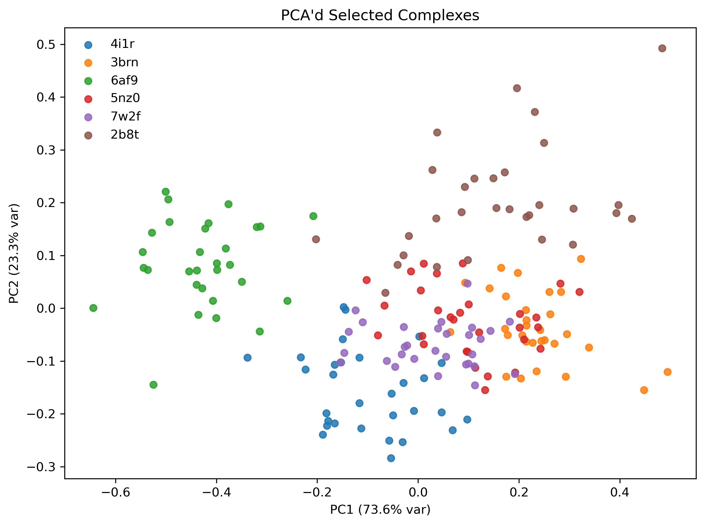
To ensure that the PCA'd embeddings actually had some signal, I plotted a 2-dimensional PCA projection for a few selected complexes. Note that there are 30 dots per complex as opposed to 300; due to compute restrictions, I calculated embeddings for every 10th frame from my snapshots, corresponding to samples every 100 ps. Clearly, dots from the same complex's trajectory are clustered, which is a good sign. Ideas of using the variance within the PCA'd dimensions as an additional feature related to entropy arise from this plot, which I ended up doing.
Unfortunately, this approach didn't pan out super nicely. There's a lot to break down here.
The associated RMSE and correlation coefficient values are as follows:
| Subset | RMSE | R |
|---|---|---|
| Train | 0.83 | 0.959 |
| Validation | 1.86 | 0.414 |
| Test | 1.93 | 0.654 |
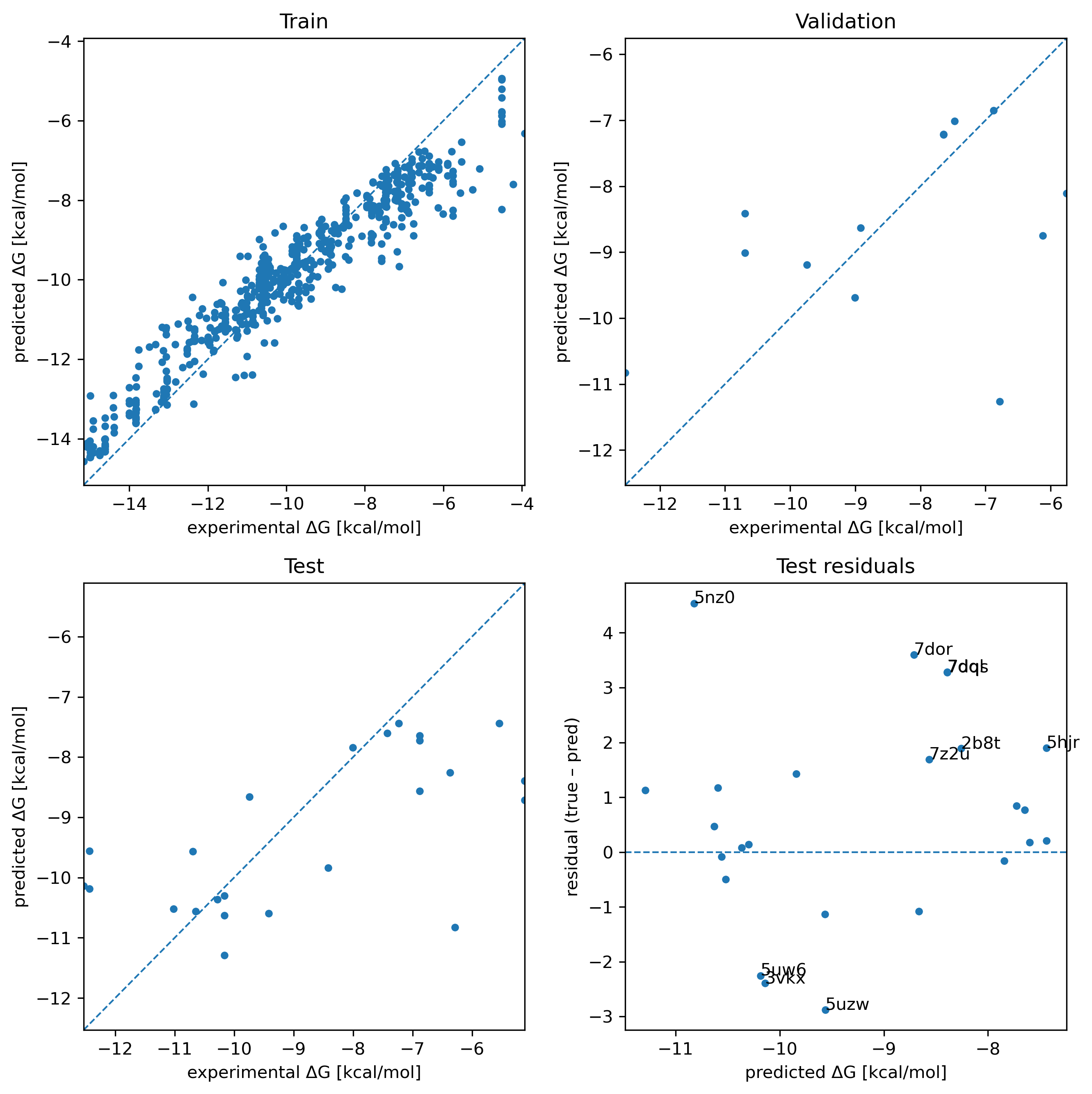
There's obviously overfitting here, but this was the result of a long sweep over loads of different hyperparameter combinations. Tuning hyperparameters to achieve closer to equal RMSE and R values across the three splits performed exceptionally badly on data from the ULVSH work. This study looked at existing experimental data for 10 targets, each with roughly 40 candidate ligands (some had a little less and some had many more). The key results are summarized in this table from the paper's SI:
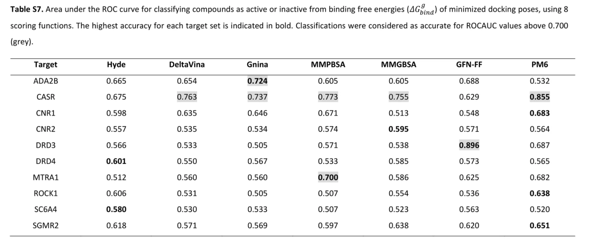
The first three scoring functions (Hyde, DeltaVina, and Gnina) are docking functions.
Our model achieved the following results on the CNR1, DRD3, MTR1A, and ROCK1 complexes from this set:
| Target | Our model | Gnina | MMGBSA |
|---|---|---|---|
| DRD3 | 0.681 (0.658) | 0.505 | 0.538 |
| CNR1 | 0.523 | 0.646 | 0.513 |
| ROCK1 | 0.555 (0.545) | 0.505 | 0.554 |
| MTR1A | 0.509 | 0.560 | 0.586 |
These results imply functionally random guessing. The values in parentheses for the DRD3 and ROCK1 targets are due to differently charged ligands among the candidates; the ligand data I trained, validated, and tested on was completely neutral.
The outcomes of these two approaches are definitely frustrating. However, I don't think the situation looks too bleak. The RMSE and R values on the PLINDER-PL50 train/validation/test split weren't too bad. Validation had poor correlation, but this looks to be largely due to a single outlier. I suspect that the small amount of data we used was a bottleneck; loosening the dataset construction guidelines to not use the strictest PLINDER split or accepting compounds with 2+ measurements (as opposed to 3+) could help.
Interestingly, the XGBoost hyperparameters that resulted in the shown predictions weighted the first 2 PCA'd ATOMICA embedding dimensions quite highly.
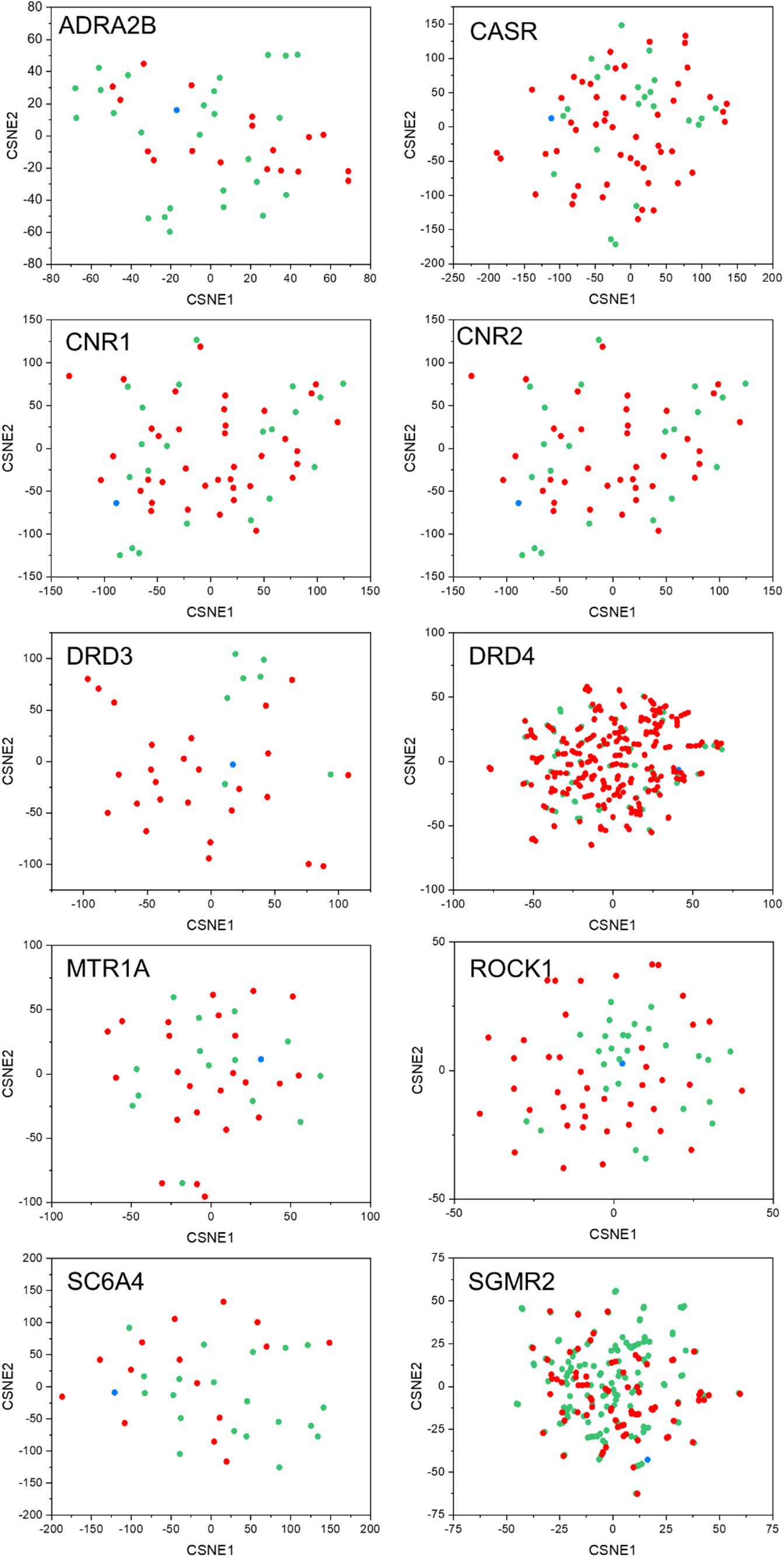
t-SNE ECFP4 descriptor projections from the ULVSH work.
While we only tested against 4 of the 10 targets in this set, the authors of the work note the following:
In most sets, inactive and active ligands do occupy very similar spaces and discriminating the two classes appears almost impossible by just looking at the 2D maps… The DRD3 set is a noticeable exception to this trend since most of the actives are clearly distinguishable from most inactive ligands in the t-SNE map.
Perhaps this implies some distributional agreement between the PCA'd ATOMICA embeddings and the ECFP4 descriptor projections. This essentially means that when projected onto two dimensions, the ECFP4 descriptors and ATOMICA embeddings produce similar point geometries/patterns. Of course, significant testing would have to be done to actually confirm or reject this suspicion.
Outlook
Broadly, I feel that a key takeaway from these efforts at filling the binding-affinity-prediction gap is that "working up" from MM/GBSA (and similar approaches) is probably not a great idea. Fundamentally, MM/GBSA-style multi-term approaches aren't guaranteed to work even at the limit where each term becomes perfect. Even if we had a really good interaction-energy predictor, the GBSA solvent model is a crude approximation of the PBSA solvent model, which is a crude approximation itself. And even if we also had a really good solvent model to use here, we'd struggle with the entropic term (several kcal/mol). And even if we had also a great way to estimate the entropic penalty, our single-trajectory MD simulation means we aren't properly accounting for ligand strain or pocket strain. In short, the list of missing things is practically endless.
Super heuristically, a better approach might be to work "top-down" from methods like FEP, which are really only limited by two things: forcefield accuracy and the amount of sampling done. Since we already know FEP is good, it seems likely that we would more easily be able to predict and interpret the effect of additional modifications and approximations.