Free-Energy Perturbation: A Pedagogical Introduction
by Corin Wagen · Mar 4, 2026
This interactive tutorial illustrates the core concepts behind free-energy perturbation (FEP) using simple 1D toy systems where we can compare numerical estimates to exact analytical results. While there's a lot that's not included in this tutorial, we hope that this helps give scientists who aren't already stat-mech experts a sense for what's going on "under the hood" in FEP.
What Problem Are We Solving?
We want to compute the free-energy difference ΔA between two thermodynamic states (0 and 1) with potential energy functions U0(x) and U1(x). In real life, these two states might be two ligands bound to a protein or two ionization states of a molecule.
The free energy A is related to the partition function Z:
A=−kBTlnZ
where Z=∫e−βU(x)dx and β=1/kBT. (T is the temperature and kB is Boltzmann's constant.)
The challenge is that we can't easily compute Z directly in complex systems. Instead, we can sample configurations from a Boltzmann distribution. FEP provides a way for us to convert these samples into an estimate of ΔA.
Let's make this concrete. We'll use harmonic oscillators for this tutorial because they have analytical solutions; the potential energy is determined by the spring constant k and the equilibrium position x0:
U(x)=21k(x−x0)2
The partition function is Z=2π/βk, giving:
A=21kBTln(2πβk)
For two oscillators with force constants k0 and k1 (same center):
ΔAexact=21kBTln(k0k1)
Use the sliders below to explore how the potentials and Boltzmann distributions change with different force constants:
Loading chart ...
The Zwanzig Equation
The Zwanzig equation (1954) gives us an exact expression for ΔA that doesn't depend on the partition function:
ΔA=A1−A0=−kBTln⟨e−β(U1−U0)⟩0
Here, ⟨⋅⟩0 denotes an ensemble average over configurations sampled from state 0.
In practice, we:
Sample configurations {xi} from the Boltzmann distribution of state 0
Compute ΔUi=U1(xi)−U0(xi) for each configuration
Estimate: ΔA≈−kBTln(N1∑ie−βΔUi)
The accuracy of the output result depends on the accuracy of the ensemble average. Try different sample sizes and resample to see how the estimate varies:
Loading chart ...
The Overlap Problem
This simple approach works well when the two states have good phase-space overlap. When the states are very different, though, sampling becomes much harder. Try increasing k1 below and see how the accuracy of the ΔA estimate changes for different sample numbers:
Loading chart ...
When the states are too different, most samples from state 0 have very high energies in state 1, leading to Boltzmann factors near zero. The average is then dominated by a few rare samples, causing high variance and unreliable estimates.
Fortunately, there's a solution. Instead of jumping directly from state 0 to state 1, we introduce intermediate states parameterized by λ∈[0,1]:
Uλ(x)=(1−λ)U0(x)+λU1(x)
For our harmonic oscillators:
Uλ(x)=21kλx2wherekλ=(1−λ)k0+λk1
Now we can compute ΔA as a sum of small steps:
ΔA=i=0∑n−1ΔAλi→λi+1
Using intermediate states allows us to compute accurate free-energy estimates even between very different states. Try adding intermediate states below and see how the estimate of ΔA changes. (You can click "Resample" to rerun the simulation.)
Loading chart ...
Adding just a few lambda windows dramatically increases the accuracy of the simulation, but there are diminishing marginal returns: once there's sufficient overlap between adjacent states, more windows just adds complexity without increasing accuracy.
Shifted Oscillators
Now let's consider oscillators with different centers.
For harmonic oscillators with the same force constant but different centers, ΔA=0 regardless of the shift (the partition function only depends on k, not x0). But the Zwanzig equation will have trouble due to poor overlap and typically predict non-zero values. Try this yourself by increasing Δx on the slider below; as before, adding lambda windows prevents poor overlap and allows us to get the correct prediction.
Loading chart ...
Real-World FEP
These toy systems illustrate some of the key concepts of FEP: small perturbations are easy to model, while larger perturbations often have insufficient phase-space overlap and require large numbers of intermediates to give reliable results. This is why relative binding affinities are so much easier to compute than absolute binding affinities, and also why small chemical perturbations are easier to handle than large chemical perturbations.
In practical FEP simulations used to compute protein–ligand binding affinity, the potential-energy function is much more complicated and it's not possible to directly sample from the Boltzmann distribution. Instead, we have to run molecular dynamics, which introduces an additional set of sampling challenges. State-of-the-art FEP engines like TMD incorporate a large number of "tricks" aimed at increasing sampling as much as possible: grand canonical Monte Carlo water sampling, local resampling, replica exchange with solute temperating, and so on.
If you're interested in trying FEP on real problems, Rowan offers self-service and managed FEP calculations designed to accelerate early-stage drug discovery.
Start running calculations in minutes!
Our platform lets you submit, view, analyze, and share calculations using cutting-edge methods trusted by hundreds of leading scientists. We give every new user 500 free credits to start, plus more every week. Making an account and running your first calculation takes only seconds: start using Rowan today!