An Introduction to Neural Network Potentials
by Ari Wagen · Dec 19, 2024
Neural network potentials (NNPs)—also called neural network interatomic potentials (NNIPs), machine-learned interatomic potentials (MLIPs), and occasionally machine-learned forcefields (MLFFs)—are machine-learned (ML) models used to approximate solution of the Schrödinger equation, which describes how systems of atoms will behave with quantum accuracy.
This article is written to serve as an introduction to NNPs for scientists without prior knowledge of the field, and it contains the following sections:
- Why NNPs Matter
- Early NNPs
- NNP Datasets
- NNP Architectures
- General Pretrained NNPs
- Benchmarking NNPs
- Applications of NNPs in Life and Materials Sciences
- Future Directions for NNPs
- How to Start Using NNPs
- How to Start Training and Fine-Tuning NNPs
Why NNPs Matter
NNPs are an emerging technology for atomistic simulation. But why do we care about simulating atoms in the first place? If we can accurately model atoms, molecules, and systems of molecules, then we can study phenomena that are too small and fast to observe by other methods and we can learn things about chemistry without having to run error-prone and expensive experiments in the real world. In theory, this should let us accelerate the pace of scientific research in important fields like drug discovery and materials science; in practice, simulating atoms turns out to be extremely difficult.
The Schrödinger equation is a quantum mechanical equation that describes the wave-like nature of electrons. When solved, this equation exactly describes the behavior of non-relativistic systems (within the Born–Oppenheimer approximation). Sadly, the solution of this equation is very complex, and systems with more than two atoms introduce many-body interactions that make analytical solutions of the equation impossible. If we treat propane's nuclei as fixed and just solve for the electronic wavefunction, it still takes 6.6 years to compute.
To model systems in a reasonable amount of time, different approximations have been made to the Schrödinger equation, leading to the creation of a number of quantum mechanics (QM) "methods," including the Hartree–Fock method, density-functional theory (DFT), Møller–Plesset perturbation theory, and coupled cluster.
These different methods are among the most complex and compute-intensive algorithms in scientific computing; but at a very high level, they can all be thought of as functions that take a list of atomic numbers and their Cartesian coordinates and return that system's energy, the energy's gradients with respect to atomic position (also called "forces"), and a number of other electronic properties including the dipole moment, excitation energies, and electron distribution (Figure 1A).
Unfortunately, these algorithms—while tractable for systems up to hundreds of atoms—are still very slow. To accelerate QM-style simulation, people have fit the potential energy surface of atomic systems to simple polynomial equations. For simple systems, this can be done very accurately, enabling much longer simulations to be run at high accuracy; this has been done for a number of systems, including hydrogen sulfide, H+H2, NaCl–H2, H2O−H2, and H+D. However, this approach becomes very complex for systems with more than a few atoms.
Advances in machine learning allow us to scale fast approximations of QM to large and complex systems. Instead of fitting a number of polynomial terms to a potential energy surface, ML models can fit millions of parameters to more complex QM data. With these models (NNPs) trained to work as functional approximators of QM, high-accuracy atomistic simulations can now be run many orders of magnitude faster than traditional QM simulations.
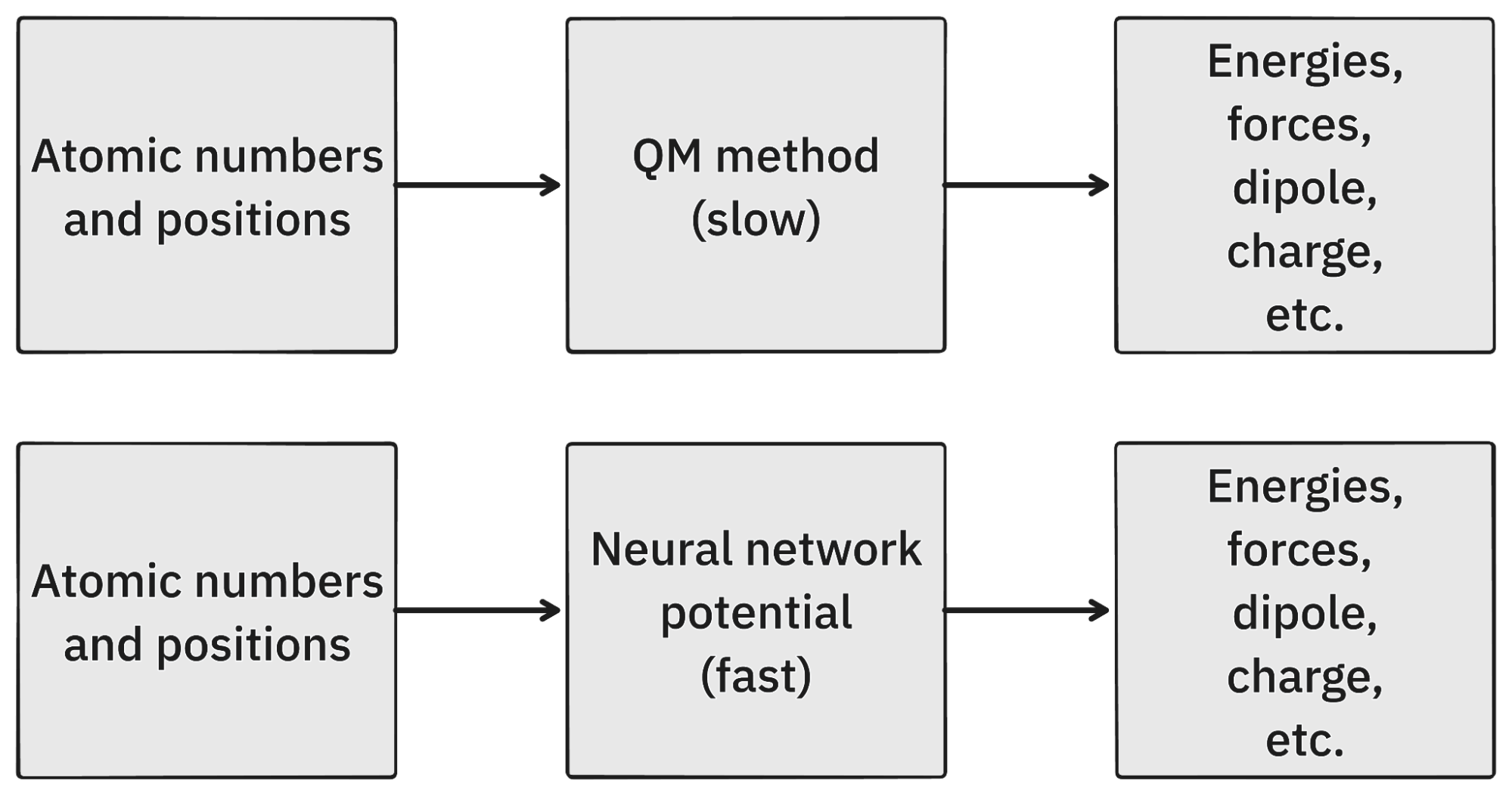
Figure 1. A simplified overview of QM and NNPs.
It's worth noting a distinction that will be important in the rest of this article. In molecular simulation, there are two types of calculations: molecular and periodic. Briefly, molecular calculations model finite molecular systems (isolated molecules or groups of molecules surrounded by a vacuum or a dielectric field) while periodic calculations model infinite systems by using a repeating unit cell, where the molecule or group of molecules "sees" itself tiled infinitely in all dimensions. Molecular and periodic QM are usually implemented in different software packages; similarly, NNPs tend to be trained on either only molecular or only periodic QM data.
There are a variety of commercial, academic, and open-source QM software packages used to run high accuracy simulations and generate training data for NNPs. These include PySCF, Psi4, CP2K, GAMESS, Gaussian, Q-Chem, FHI-aims, Schrödinger's Jaguar, FACCTs' ORCA, TURBOMOLE, PetaChem's TeraChem, NWChem, Quantum Espresso, and VASP.
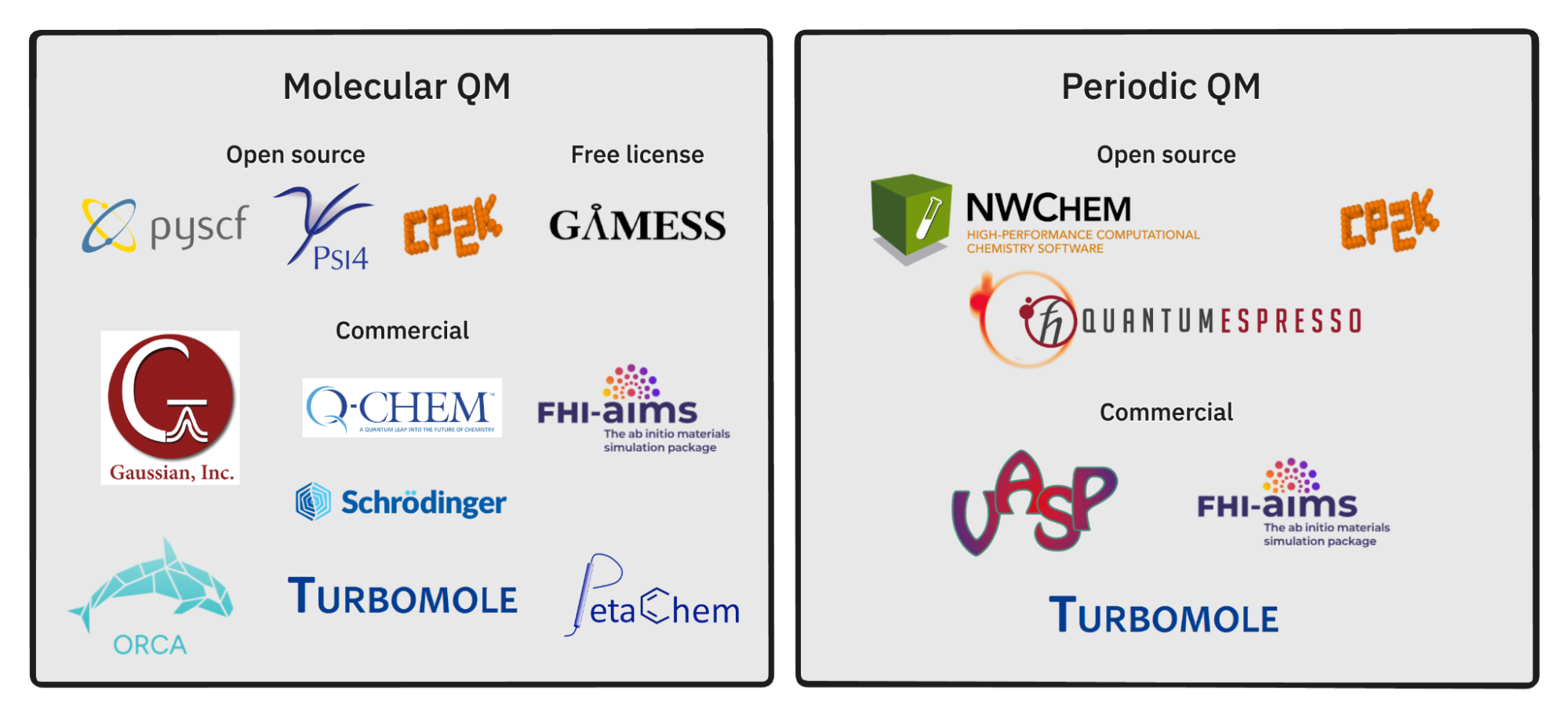
Figure 2. An overview of widely-used commercial, academic, and open-source QM software packages. Some software packages can run both periodic and molecular calculations; in these cases, we've used our discretion in assessing which usage dominates per package.
QM-style simulations aren't the only way to simulate systems of atoms. Molecular mechanics (MM) is an approach to simulation that employs parametric energy-evaluation schemes called forcefields. These forcefields can get quite complex, sometimes including terms for angle stretches, dihedral rotations, van der Waals forces, polarizability, and more. Despite this complexity, forcefields are typically limited to simple functional forms like polynomials, sines & cosines, and other easily computable expressions.
The simplicity of these functional forms allows for the efficient simulation of large systems over long time scales. MM methods are commonly used for molecular dynamics (MD) and free-energy-perturbation studies, especially to model protein–ligand interactions or study conformational motion in biomolecules. However, MM forcefields are generally less accurate and less expressive than QM methods, which can lead to poor accuracy. One of the major goals of NNPs is to scale the high precision of QM-based calculations to the important workflows for which forcefields are typically used today.
To learn more about QM and MM methods, we recommend the following resources:
- Chris Cramer's computational chemistry videos from his University of Minnesota course, which provide a thorough introduction to QM methods
- Corin Wagen's post on how compute-intensive QM is
- Corin Wagen's post on the distinction between molecular and periodic calculations
- Dakota Folmsbee and Geoffrey Hutchison's paper comparing the ability of different MM and QM methods to rank conformers by relative energy
Early NNPs
The first1 modern NNP was published by Jörg Behler and Michele Parrinello in a 2007 Phys. Rev. Lett paper studying bulk silicon. This NNP used a simple architecture and was trained on 8,200 DFT energies. Unlike most QM engines, the architectures of NNPs (including this first NNP) make them able to handle both molecular and periodic systems.
Early researchers in this field trained new NNPs for every system under study. For example, in 2012, Behler and coworkers published an NNP trained on the water dimer. Their NNP learned the full potential energy surface of the water dimer in good agreement with their DFT calculations.
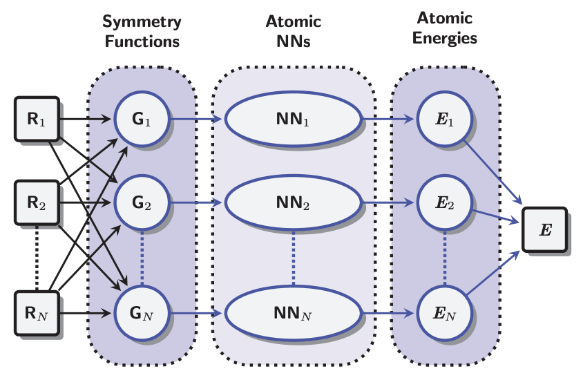
Figure 3. The basic NNP architecture used by both Parrinello (2007) and Behler (2012). Atomic coordinates are fed through symmetry functions and then "fed forward" through a number of "hidden" matrix layers to produce per atom energies. These per atom energy contributions are summed to yield a total energy prediction. This illustration is taken from Figure 1 of Behler 2012.
In 2017, building on the Behler and Parrinello symmetry functions and architecture, Justin Smith, Olexander Isayev, and Adrian Roitberg released ANI-1, a general pretrained NNP. The ANI-1 dataset comprised "~17.2 million conformations generated from ~58k small molecules." These atoms contained up to 8 heavy atoms and were made up of the elements H, C, N, O. In the paper, the authors then go on to show that the ANI-1 NNP can be used to make accurate predictions on systems containing more than 8 heavy atoms, showing good agreement with QM potential energy surfaces. This result showed that NNPs could generalize to unseen topologies: instead of training a new NNP for every system of interest, scientists could use a single pretrained NNP to model unseen molecules with good accuracy, so long as the model had been trained on similar types of molecules.
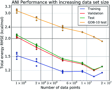
Figure 4. ANI-1 showed that NNPs could generalize across topologies at scale. This illustration is taken from figure 3 of Smith et al. 2017 (the ANI-1 paper).
NNP Datasets
Before continuing to look at the inner workings of NNPs, it's worth taking some time to look at the data these models are trained on. NNPs are trained to recreate the results of QM software. This means that given some list of atomic numbers and positions, NNPs should be able to predict energies, forces, etc. that closely match those predicted by QM.
To match the breadth of QM, people training NNPs spend a lot of time thinking about how to sample molecular space well to ensure that NNPs will be able to handle all kinds of structures. In this vein, Jean-Louis Reymond and co-workers have worked on a series of databases that enumerate all chemically feasible molecules under sets of constraints:
- GDB-11 (paper): a dataset enumerating small organic molecules up to 11 atoms of C, N, O and F.
- GDB-13 (paper): a dataset enumerating small organic molecules up to 13 atoms of C, N, O, S and Cl
- GDB-17 (paper): a dataset enumerating 166.4 billion molecules of up to 17 atoms of C, N, O, S, and halogens.
These enumerated structure databases have been used as the starting point for QM databases, including:
- QM-7 (download): a dataset of molecular DFT calculations performed on 7,165 small organic molecules from the GDB-13 database
- QM-9 (paper): a dataset of molecular DFT calculations performed on every structure containing up to 9 heavy atoms in GDB-17
The Materials Project (paper, website) was started in the 2010s to be an open repository for computational data on materials. This dataset was originally centered around structures relevant to battery research, but it has since expanded. The Materials Project is the basis of a widely used QM dataset:
- MPtrj, or MPtraj (download): a dataset of 145k periodic DFT relaxations (nearly every compound in the Materials Project)
To help create datasets that could be used for catalyst design and optimization, Meta and Carnegie Mellon teamed up to start the Open Catalyst Project. The Open Catalyst Project generated QM datasets that included structures relevant to surface catalysis, including:
- Open Catalyst 2020, or OC20 (paper): a dataset of 1.2 billion periodic DFT relaxations "across a wide swath of materials, surfaces, and adsorbates"
- Open Catalyst 2022, or OC22 (paper): a dataset of 62k periodic DFT relaxations focused on oxide chemistries
In 2023, Meta and Georgia Tech collaborated to work on direct air capture, releasing:
- OpenDAC 2023, or ODAC23 (paper, download): a dataset of "170k [periodic] DFT relaxations involving metal organic frameworks (MOFs) with carbon dioxide and water adsorbates"
In 2024, Meta continued this work, releasing:
- Open Materials 2024, or OMat24 (paper, download): a dataset of 118 million periodic DFT calculations on inorganic bulk materials with a focus on non-equilibrium structures
In 2023, Peter Eastman teamed up with others to generate very accurate QM data that would enable ML models to predict drug-like small molecule and protein interactions, leading to:
- SPICE (paper): a dataset of 1.1 million molecular DFT calculations on small molecules, dimers, dipeptides, and solvated amino acids
- SPICE 2.0 (download): an expanded version of SPICE with 2 million molecular DFT calculations
Finally, another dataset that sees frequent use is Miguel Marques and coworkers':
- Alexandria (PBE) (paper, download): a dataset of over 2.5 million periodic DFT relaxations on materials
- Alexandria (PBEsol) (paper, download): a dataset of 175k periodic DFT relaxations on materials
Which should not be confused with:
- Alexandria (paper, download): a dataset of 2,704 molecular DFT relaxations on organic and inorganic molecules
To read more about datasets that have been created for training NNPs, we recommend:
- Arif Ullah's list of molecular datasets on Github and the accompanying review
- Justin Smith and Los Alamos National Laboratory researchers' recent paper, "Data Generation for Machine Learning Interatomic Potentials and Beyond"
NNP Architectures
In NNPs, molecular structures are commonly represented as graphs. In this representation, each atom corresponds to a node (or "point") in the graph, and edges connect an atom to its neighboring atoms within a specified cutoff radius. This cutoff defines which atoms are considered "neighbors," ensuring that each atom primarily interacts only with those in its local vicinity. This principle is known as the "locality assumption": the idea that an atom's environment—and hence its contribution to the system's energy—depends predominantly on atoms within a local spherical region around it.
In some NNPs, these local environment representations are then transformed by symmetry functions (more on this in the "Ensuring Invariance/Equivariance" section below). After obtaining these local representations, the neural network processes them through a series of hidden layers to produce atomic energy contributions. Finally, these per-atom energy contributions are summed across all atoms, resulting in a single total energy prediction for the entire structure.
From this basic architecture, NNP architectures have branched out in several directions. Four main themes have emerged: the addition of global inputs, the tension between fully enforcing equivariance and simplifying models for speed, the tradeoff between predicting forces directly and calculating them as derivatives of the potential energy, and the question of how to best handle long-range interactions.
Adding Global Inputs
Some models incorporate global parameters, such as total charge or thermodynamic conditions, to improve predictions beyond neutral, equilibrium scenarios. For example, in MEGNet (2019), Shyue Ping Ong and colleagues input temperature, pressure, and entropy alongside atomic numbers and positions to better predict materials properties. Oliver Unke, Klaus-Robert Müller, and coauthors give SpookyNet (2021) total system charge and multiplicity, enabling it to distinguish ionic and radical states formed from the same atoms. Other models have since followed SpookyNet's approach, including Olexandr Isayev's group's AIMNet2 (2023).
Ensuring Invariance/Equivariance
"Equivariance" means that if you transform the input of a function, the output changes in a predictable way. "Invariance' means that if you transform the input, the output stays exactly the same. With NNPs, scalar predictions like total energy ought to be invariant; if you rotate a system, its total energy shouldn't change. On the other hand, vector predictions like forces and dipole vectors ought to be equivariant; if you rotate a system, its dipole vector should rotate too.
Different NNP architectures handle questions of symmetry and equivariance very differently. At one extreme, a totally unconstrained NNP that can employ any sort of features is extremely expressive, but might struggle to learn the correct symmetry properties of a system—it's generally quite bad when rotating a molecule changes the output of a calculation. On the other end of the spectrum, an NNP that operates only on invariant features (like Behler–Parrinello symmetry functions) will have the correct rotational invariance, but might struggle to achieve sufficient expressivity to describe chemistry accurately. Equivariant architectures based around spherical harmonics and tensor products (often using packages like Mario Geiger and Tess Smidt's e3nn) inherently produce NNPs with the correct symmetries, but the additional mathematics required for training and inference generally makes these networks substantially slower. Significant work has been put into both optimizing these tensor operations, but non-equivariant models still remain substantially faster and can often learn approximate equivariance through train-time data augmentation.
Before 2019, most architectures built on Behler–Parrinello symmetry functions, which are invariant. In NEquip (2021), Simon Batzner, Boris Kozinsky, and colleagues enforce equivariance by restricting operations to equivariant spherical harmonics (using e3nn), increasing data efficiency over older Behler–Parrinello models. Stephan Günnemann's group's GemNet (2021) employs simpler spherical representations to ensure equivariance. Other methods approach equivariance differently, such as Equiformer (2022) by Yi-Lun Liao and Tess Smidt, which uses a transformer-like structure, and So3krates (2022) by J. Thorben Frank, Oliver Unke, and Klaus-Robert Müller, which introduces "spherical harmonic coordinates."
Other architectures opt to "teach" NNPs equivariance by rotationally augmenting data during training rather than strictly enforcing it, resulting in faster inference and reduced memory usage. Sergey Pozdnyakov and Michele Ceriotti describe this approach in "Smooth, exact rotational symmetrization for deep learning on point clouds" (2023). Mark Neumann and coworkers' Orb (2024) rotationally augments its data during training, increasing inference speed by "3–6x." Similarly, Eric Qu and Aditi Krishnapriyan's EScAIP (2024) uses rotational data augmentation to increase inference speed and reduce memory costs, achieving state-of-the-art performance on multiple datasets.
Predicting Forces
"Forces" are the derivatives of a system's total energy with respect to atomic positions. Accurate force predictions are essential for running simulations like relaxations or molecular dynamics. Any method—whether QM, MM, or NNPs—must be capable of predicting forces accurately. Fortunately, neural networks excel at this task. As Behler and Parrinello noted in their 2007 paper: "Once trained, the atomic coordinates are given to the NN and the potential energy, from which also forces can be calculated analytically, is received."
Analytical force calculation through a neural network is enabled by libraries like PyTorch, using automatic differentiation to compute derivatives. This approach is referred to as "conservative" because the predicted forces respect the conservation of energy.
Since analytical differentiation makes inference slower, some architectures opt to predict forces directly as additional model outputs. This requires training the neural network to predict both energies and forces and eschews the differentiation step, roughly doubling the speed of NNP inference. However, this "non-conservative" method can lead to unstable simulations, as highlighted in Filippo Bigi and others' recent "The dark side of the forces: assessing non-conservative force models for atomistic machine learning."
Handling Long-Range Interactions
The locality assumption—that an atom's energy contribution depends primarily on its neighbors within a certain radius of it—fails to capture long-range interactions like electrostatic energy and van der Waals forces.
To make some of these forces learnable, Kristof T. Schütt, Alexandre Tkatchenko, Klaus-Robert Müller, and others released SchNet (2017), an NNP that uses a graph-based, "message-passing" architecture as introduced by Justin Gilmer and coworkers' "Neural Message Passing for Quantum Chemistry" (2017). In SchNet's framework, each atom and its neighbors (defined by a local cutoff radius) are represented as nodes and edges in a graph. Through iterative message passing steps, each atom's embedding is updated based on information propagated from its immediate neighbors, allowing the network to build increasingly accurate and context-aware representations of local chemical environments that reach beyond each atom's immediate neighbors. Message passing, used to propagate local information through graphs, can mitigate strict locality but often slows models. Ilyes Batatia, Gábor Csányi, and others speed it up in MACE (2023) by passing fewer higher-order messages, while Seungwu Han and others' SevenNet (2024) parallelizes many of NEquip's message-passing steps. Some architectures, like Allegro (2023) from Albert Musaelian, Simon Batzner, Boris Kozinsky, and collaborators, abandon message passing entirely for better scalability.
Other architectures have added physical equations to capture the effect of these long-range interactions. John Parkhill's group's TensorMol-0.1 (2018) divides total energy predictions into short-range embedded atomic energy, electrostatic energy, and van der Waals energy components. To predict the total energy of a structure, TensorMol-0.1 uses physical equations to calculate electrostatic energy and van der Waals energy before using a standard NNP architecture to predict the remaining energy terms. Other architectures, including Jörg Behler and others' "fourth-generation high-dimensional" NNP (2021), Schrödinger's "QRNN" (2022), and Dylan Anstine, Roman Zubatyuk, and Olexandr Isayev's AIMNet2 (2023), have also adopted this approach, combining machine-learned short-range terms with physics-based long-range components to reduce the need for extensive message passing.
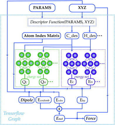
Figure 5. By calculating electrostatics and van der Waals forces with simple physical equations, TensorMol-0.1 is able to accurately model long-range interactions while maintaining the speed of other NNPs. This illustration is taken from figure 1 of Yao et al. 2018 (the TensorMol-0.1 paper).
To read more about the development of NNP architectures as well as current problems and their potential solutions, we recommend reading:
- YuQing Xie and others' "The Price of Freedom: Exploring Tradeoffs between Expressivity and Computational Efficiency in Equivariant Tensor Products"
- Yuanqing Wang and others' "On the design space between molecular mechanics and machine learning force fields"
- Filippo Bigi, Marcel Langer, and Michele Ceriotti's "The dark side of the forces: assessing non-conservative force models for atomistic machine learning"
- Jörg Behler's review "Four Generations of High-Dimensional Neural Network Potentials"
- Dylan Anstine and Olexander Isayev's "Machine Learning Interatomic Potentials and Long-Range Physics"
- Corin Wagen's "Long-Range Forces and Neural Network Potentials"
General Pretrained NNPs
Traditionally, using an NNP required generating data and training a new model for each new system under study. To help bring NNPs to bear on more problems, a growing number of academic labs, startups, and big tech firms have released general pretrained NNPs (sometimes called "foundation models"). These models are trained once on extensive, diverse datasets, with the goal of capturing broad patterns in atomic behavior. The resulting NNPs can then be used to make predictions on novel systems within a similar domain, drastically reducing setup time and effort, or fine-tuned to achieve better data efficiency for specific problems. However, an NNP's efficacy is only ever as good as the scope and quality of its training data, its architecture, and its training procedure.
Olexander Isayev's group and Adrian Roitberg's group collaborated on the ANI series of models, including:
- ANI-1x (paper): a pretrained NNP focused on drug-like molecules, supporting H, C, N, and O
- ANI-1ccx (paper): a pretrained NNP trained on the ANI-1x dataset and finetuned on CCSD(T) data, supporting H, C, N, and O
- ANI-2x (paper): a pretrained NNP focused on drug-like molecules, supporting H, C, N, O, F, Cl, and S
Since then, the Isayev group has developed the AIMNet architecture, most recently releasing:
- AIMNet2 (paper, GitHub): a DFT-quality pretrained NNP focused on main group organic molecules supporting "14 chemical elements in both neutral and charged states"
Gábor Csányi's group has released pretrained models using the MACE architecture, including:
- MACE-MP-0 (paper, GitHub): a pretrained NNP for materials trained on the MPtrj dataset
- MACE-OFF23 (paper): a pretrained NNP trained for organic molecules trained on the SPICE dataset (note: MACE-OFF23 is not licensed for commercial usage)
Other academic labs working on NNPs have released pretrained models as well, including:
- SO3LR (paper, GitHub): a pretrained NNP for organic molecules from Alexandre Tkatchenko's group
- AIQM2 (paper): a pretrained NNP for organic molecules from Pavlo Dral's group
- SevenNet (paper, GitHub): a pretrained NNP for materials trained on MPtrj from Seungwu Han's group
- M3GNet (paper, GitHub): a pretrained NNP for materials trained on MPtrj from Shyue Ping Ong's group
- CHGNet (paper, GitHub): a pretrained NNP for materials trained on MPtrj from Gerbrand Ceder's group
Orbitals Materials, a startup using NNPs to design advanced green materials, has also released permissively-licensed pretrained NNPs, including:
Many big tech firms have also released pretrained NNPs for different applications, including:
- BAMBOO (paper, GitHub): a pretrained NNP for lithium battery electrolytes from ByteDance
- OMat24 (paper, Hugging Face): a pretrained NNP for materials trained on the OMat24 dataset, MPtrj, and Alexandria from Meta
- MatterSim (paper, GitHub): a pretrained NNP for materials trained on data from different temperatures and pressures from Microsoft
Google trained an NNP for materials discovery applications, but they didn't release the pretrained model:
(And while we're talking about big tech, Apple has a paper out on using machine learning to generate conformers.)
For a more exhaustive list of pretrained NNPs, we recommend looking at:
- Jin Xiao's list of neural network models for chemistry
Benchmarking NNPs
QM and MM methods rely solely on physical or physically-motivated equations, allowing them to generalize effectively to new atomic systems. NNPs, however, are empirical. To quote Yuanqing Wang:
Conceptually, to accurately fit energies and forces on all chemical spaces is no different than having the MLFF model able to solve the Schrödinger's [sic] equation, which seems impossible, judging from the no free lunch theorem. To this end, QM datasets are always curated with biases, in terms of the coverage on chemical spaces and conformational landscape.
An NNP trained exclusively on inorganic materials is unlikely to make accurate predictions for organic structures. Researchers in this field use various tools and strategies to improve the robustness and utility of NNPs, but rigorous benchmarking is essential to ensure their predictions are decision-worthy. To evaluate the performance of different NNPs on specific tasks, researchers and users depend on standardized benchmarks.
In silico benchmarks evaluate NNP predictions against high-level QM results. Energy benchmarks, for instance, compare the relative energy outputs of NNPs to high-accuracy QM energy values. Some energy benchmarks include:
- GMTKN55 (paper, download): a high-accuracy molecular benchmark that measures basic properties, reaction energies, and noncovalent interactions
- TorsionNet500 (paper): a benchmark comprising 500 diverse torsion profiles
Other benchmarks assess NNP predictions of forces, dipoles, and other electronic properties, comparing them directly to high-level QM results. Some studies go further, using higher-level benchmarks to compare NNP-predicted potential energy surfaces, radial distribution functions, and folded protein structures against those computed using QM or MM methods.
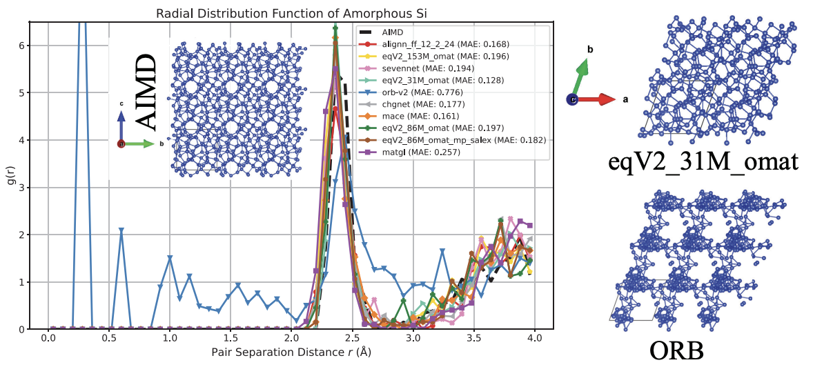
Figure 6. The radial distribution function of amorphous Si as predicted by a number of NNPs trained on materials versus the AIMD prediction (vdW-DF-optB88). This illustration is taken from figure 4 of Wines and Choudhary (the CHIPS-FF paper).
One goal of benchmarking NNPs is to assess whether or not they can support stable molecular dynamics (MD) simulations. In "Forces are not Enough: Benchmark and Critical Evaluation for Machine Learning Force Fields with Molecular Simulations," Rafael Gomez-Bombarelli, Tommi Jaakkola, and colleagues argue that strong energy and force benchmark results alone are insufficient to guarantee MD stability, and instead benchmark different NNPs by directly running MD simulations and checking for instability.
Experimental benchmarks evaluate NNP predictions against experimental data. Since it's impossible to directly measure the total QM energy of a system to validate single-point energy predictions, these benchmarks are all higher level. Common experimental benchmarks include tests for crystal structure stability ranking and the reproduction of protein crystal structures. For example, X23 is a benchmark measuring molecular crystal cell volume and lattice energy predictions.
Benchmarking NNPs is still a very active and fast-moving area of research.
To compare the performance of NNPs on different benchmarks, we recommend checking out:
- The Materials Project's Matbench Discovery, which ranks NNPs "on a task designed to simulate high-throughput discovery of new stable inorganic crystals"
- Ari Wagen's NNP Arena, which compares the GMKTN55 performance of NNPs to QM methods
- Daniel Wines and Kamal Choudhary's CHIPS-FF, which focuses on benchmarking " complex properties including elastic constants, phonon spectra, defect formation energies, surface energies, and interfacial and amorphous phase properties"
- Yuan Chiang and Philipp Benner's MLIP Arena, which ranks NNPs' homonuclear diatomics and thermal conductivity predictions
- The Open Catalyst Project's OC22 Leaderboard, which measures NNPs' ability to learn the OC22 dataset
Applications of NNPs in Life and Materials Sciences
When applying NNPs to problems, they can be thought of as faster QM methods or as more accurate MM methods. As NNPs become both faster and more accurate, they promise to prove valuable in use cases that currently rely on both QM and MM.
In drug discovery, QM methods are used to generate and score conformers, compute charges, run torsional scans, predict pKa, compute bond-dissocation energies, search for tautomers, model reactivity, predict crystal structure stability, and more (this list is taken from Corin Wagen's "Quantum Chemistry in Drug Discovery"). NNPs are already being used for all of these tasks, helping researchers answer questions about structures in a fraction of the time that QM previously needed.
MM methods, on the other hand, are often used to run molecular dynamics simulations and free energy perturbation on systems consisting of e.g. a protein, a drug-like small molecule, and solvent molecules. NNPs promise to prove useful in these cases, but the size of the systems being studied as well as the length of complexity of the simulations mean that NNPs aren't yet seeing much production use in these areas today.
In materials science, a number of startups, including Orbital Materials, cusp.ai, and Entalpic, are training NNPs to predict materials properties. Academic labs and big tech have also developed NNPs with diverse applications in mind, including:
- Developing lithium battery electrolytes
- Discovering sorbents for direct air capture
- Designing low-cast catalysts "for use in renewable energy storage"
Future Directions for NNPs
To read about future directions for NNPs, we recommend reading:
- Timothy Duignan's "The Potential of Neural Network Potentials"
- Abhishaike Mahajan's podcast with Corin and Ari Wagen "Can AI improve the current state of molecular simulation?"
- Simon Barnett and John Chodera's "Neural Network Potentials for Enabling Advanced Small-Molecule Drug Discovery and Generative Design"
How to Start Using NNPs
You can run AIMNet2 and OMat24 through the Rowan platform or API. Rowan makes it easy to run molecular simulation jobs with a simple GUI and cloud based computing. Rowan offers 500 free credits on sign up, and an additional 20 credits each week:
Many pretrained NNPs have simple tutorials attached to their GitHubs. We'd suggest starting with one of the following models:
- AIMNet2 (GitHub): a DFT-quality pretrained NNP for organic molecules
- MACE-MP-0 (GitHub): a pretrained "foundation model for atomistic materials chemistry"
- Orb-v2 (GitHub): a fast, scalable pretrained NNP for materials
To get the best performance out of an NNP, it's important to run it on a GPU. If you don't have a GPU sitting around at home, that's ok! You can quickly run code on cloud GPUs with Modal, which gives users $30 worth of free credits each month:
To run molecular dynamics with a neural network potential, see:
- The GROMACS page on NNPs, which includes an example script incorporating ANI-2X
- OpenMM-ML, which lets you use ANI-1ccx, ANI-2x, or MACE-OFF23 to run MD simulations with Open MM (note: MACE-OFF23 is not licensed for commercial usage)
How to Start Training and Fine-Tuning NNPs
If you want to train your own NNP, we recommend starting with:
- The MACE architecture and its training documentation
- TorchANI's "Train Your Own Neural Network Potential" guide
If you want to finetune a pretrained NNP with your own dataset, we'd recommend checking out:
- Orb-v2's example code for finetuning
- The finetuning documentation for the second-generation MACE-MP-0b models
Thanks to Timothy Duignan, Mark Neumann, Corin Wagen, Jonathon Vandezande, and Eli Mann for reading drafts of this piece and providing valuable feedback. Any errors are mine.
- Or, at least, one of the first.


