How to Run the OMol25/UMA Models

by Corin Wagen · May 30, 2025

Meta's recent release of the OMol25 dataset and associated models makes it possible to run high-accuracy simulations without needing massive computing resources or specialized software. Last week, we wrote about the dataset, the models, and the effect that this was having on our users' research, and we've only heard more success stories since then.

There's a lot of demand for these models, but getting started with scientific simulation can be intimidating. Over the past few weeks, we've received a lot of questions about how scientists can use these models for their own research. In this post, we provide step-by-step tutorials on how to run the OMol25/UMA models, both locally and through Rowan's cloud chemistry platform.

Running Locally

1. Get Access To UMA/OMol25 Through HuggingFace

The OMol25 page on Hugging Face.

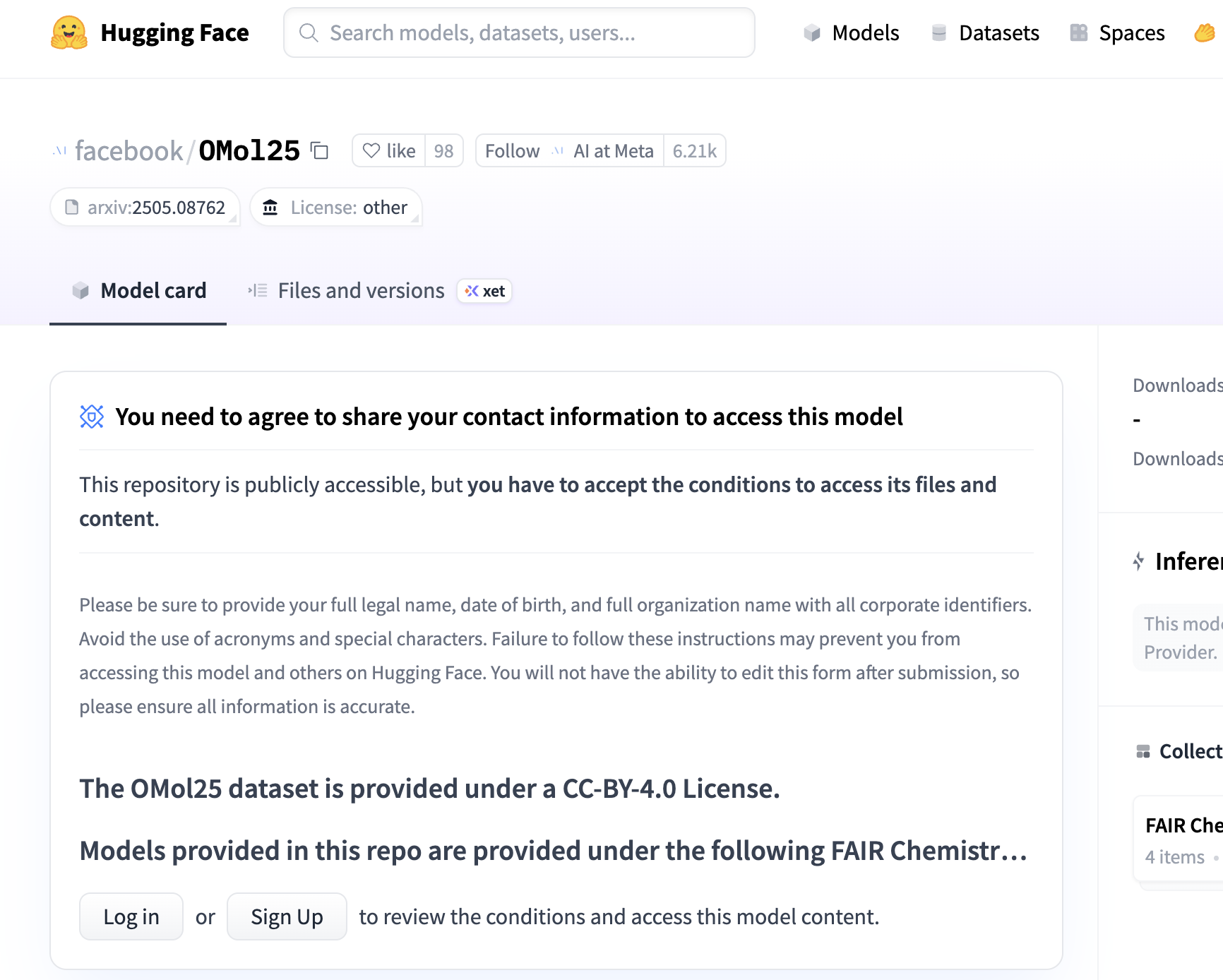
The model weights are stored on HuggingFace, but you have to request access and agree to the FAIR chemistry license, after which your request will be reviewed. Here's the link to OMol25, and here's the link to UMA.

If you're granted access, you can then download the model weights.

2. Install `fairchem-core` and `ase`

pip install ase
pip install fairchem-core

To run these calculations, install fairchem-core and ase (the Atomic Simulation Environment) from the Python Package Index.

3. Initialize the NNP

from ase.io import read
from fairchem.core import FAIRChemCalculator
from fairchem.core.units.mlip_unit import load_predict_unit

# to use an eSEN model:
esen_predictor = load_predict_unit(
    path="esen_sm_conserving_all.pt",
    device="cpu",
)

esen_calculator = FAIRChemCalculator(esen_predictor)

# to use an UMA model:

uma_predictor = load_predict_unit(
    path="uma-s-1.pt", 
    device="cuda",
        inference_settings="turbo", # optional ("turbo" accelerates inference but locks predictor to first system size it sees)
)
uma_calculator = FAIRChemCalculator(
    uma_predictor,
    task_name="omol", # options: "omol", "omat", "odac", "oc20", "omc"
)

Once the packages are installed, import them in Python and initialize a FAIRChemCalculator object using the model weights. (You'll need to change the path to match wherever you downloaded the weights.)

4. Build an `ase.Atoms` Object

atoms = read('benzene.xyz')  # or create ASE Atoms however you want
atoms.info = {"charge": 0, "spin": 1}

Structures can be loaded by creating an ase.Atoms object, which supports a variety of common filetypes. Full details about the different ways to create an ase.Atoms objects can be found in the ASE documentation.

5. Compute The Energy

atoms.calc = esen_calculator
energy_eV = atoms.get_potential_energy()
print(energy_eV) # -6319.18481262752

Finally, the FAIRChemCalculator can be associated with the Atoms object and get_potential_energy() can be called. This function uses the provided calculator to compute the single-point energy of the molecule, which is returned in eV.

The FAIRChemCalculator acts like any other calculator in ASE, making it possible to use this for geometry optimizations, molecular dynamics, and more.

Running Through Rowan

To quickly use the Meta models for high-level workflows, calculations can also be run through Rowan. Creating an account on Rowan is completely free and can be done using any Google-managed email account; create an account here.

1. Choose Workflow

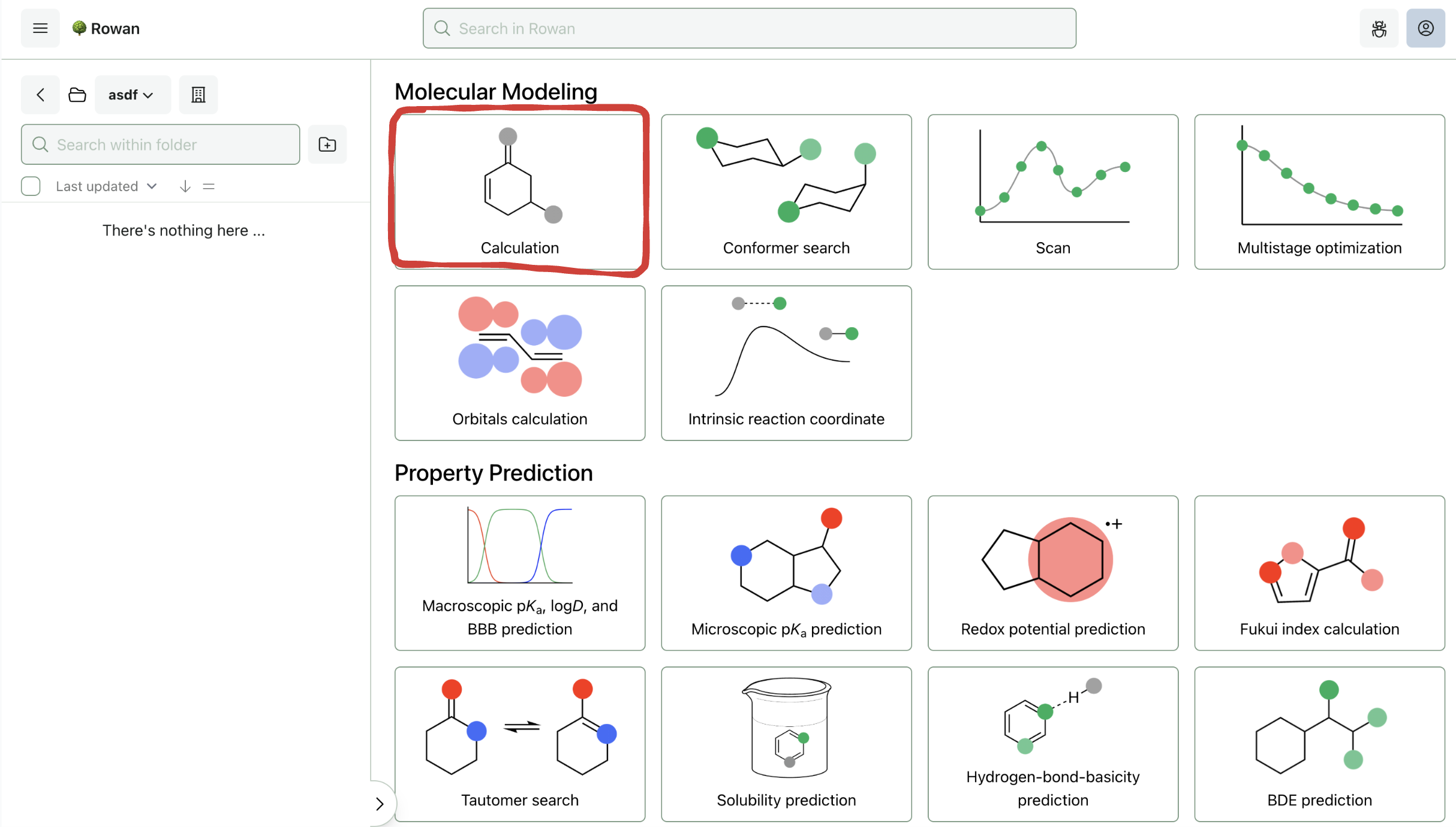
Selecting the Basic Calculation workflow.

Once you sign in to Rowan, you can select which workflow you want to run. Here, we'll run a geometry optimization followed by a frequency calculation, both of which are accessed through the "Basic Calculation" workflow.

2. Input Molecule

Inputting a sucrose molecule.

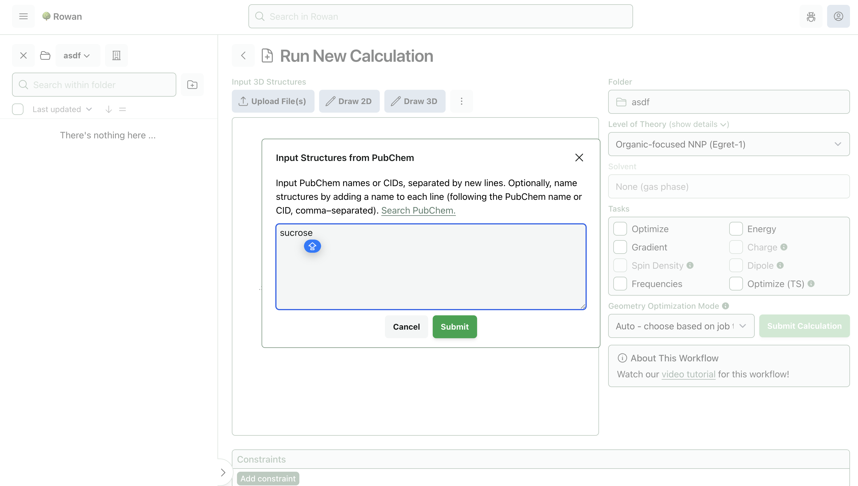
Molecules can be loaded into Rowan by name, by SMILES, by input file, or through our provided 2D and 3D editors. Here, we'll input sucrose by name.

3. Select Level of Theory

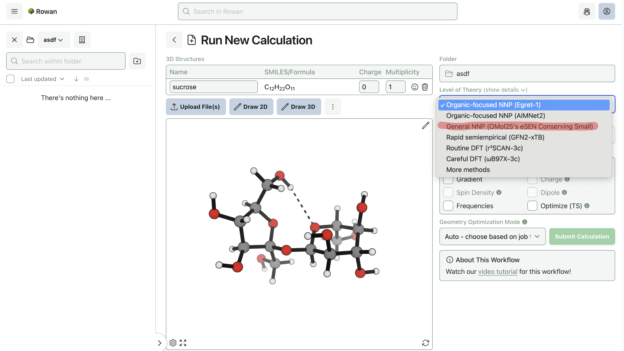
Selecting the right level of theory.

To run a calculation using the Meta models, select the model from the “Level of Theory” dropdown menu. For now, Rowan only supports Meta's small eSEN model with conservative forces; more models will be added in the future.

4. Run Calculation

The finished calculation results.

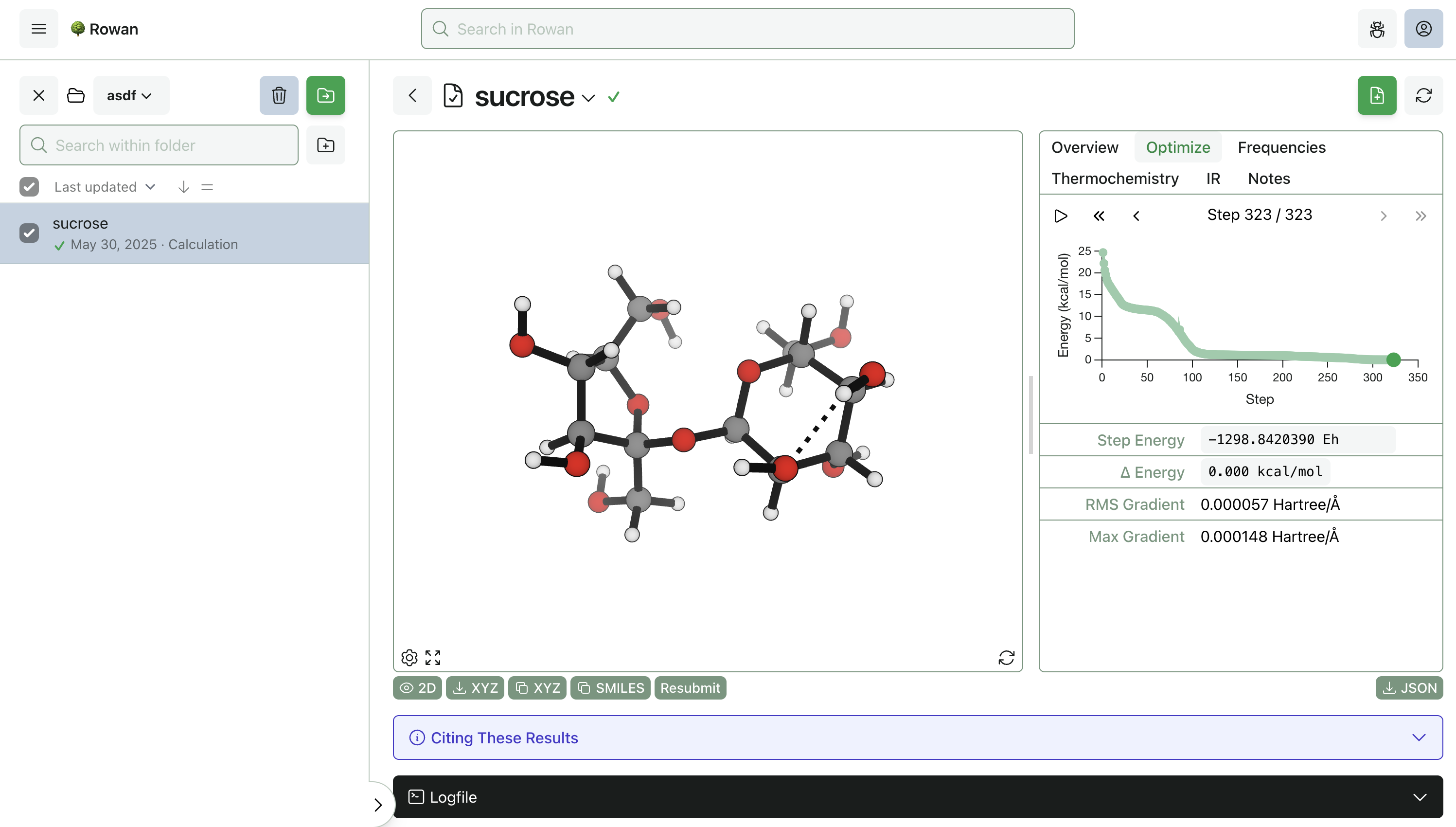
Once you click “Submit Calculation,” we'll allocate a cloud GPU and start running the calculation. Results will start streaming to your browser almost immediately, and the output structures can be viewed, analyzed, and downloaded for further use.

Here, the optimization took 323 steps to complete and finished in 84 seconds (including the frequency calculation). Thermochemistry, vibrational frequencies, optimization steps, and overall calculation statistics can be viewed by navigating around the output page. Any optimization step can be resubmitted for further calculations, including scans, transition-state searches, intrinsic reaction coordinate calculations, and property-prediction workflows.