Optimization is fundamental to many fields, but optimal optimization is difficult. For molecules, we are often interested in minima on the potential-energy surface (PES), and we use the resulting minima for property prediction. However, molecules exist in 3Natoms-dimensional space (each atom has three degrees of freedom: x, y, and z), and visualizing this complexity is difficult. To simplify, we often draw 2D surfaces, removing all the complexity and making it appear as though optimization is simple since we can see the entire surface. However, in most optimizations, the hypersurface is unknown, and in chemistry, evaluation of points and derivatives on the PES can be incredibly expensive. Thus, it is important to take as few steps as possible while attempting to find the minima.
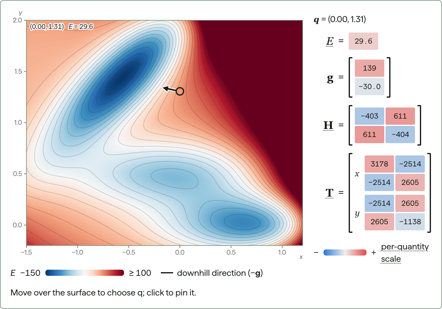
This blog introduces some of the difficulties related to optimization using a series of minigames on the Müller–Brown PES. Each minigame starts with the standard Müller–Brown surface, which stays hidden until you find all of its minima or transition states (or click "Show surface" to peek). Clicking "Random surface" generates a new surface with a different arrangement of wells to help illustrate the difficulties.
Direct search (energies only)
Below is a Müller–Brown surface; locate the three minima on the PES using the fewest possible clicks.
Loading ...
Several algorithms have been developed for finding minima when only the value (in our case, the energy) is known, including Nelder–Mead (downhill simplex) and Luus–Jaakola.
Gradient descent (local info only)
Finding minima without any direction can be difficult. In quantum chemistry, computing gradients usually incurs only a small additional cost beyond computing the energy (typically taking about the same time as one SCF cycle in DFT or a backward pass in conservative NNPs). The additional information they provide is well worth the cost. Try finding the three minima on the Müller–Brown surface with only information about the energy and gradient.
Loading ...
The gradient tells us which direction to step each time but not how far to step, since the slope alone doesn't tell us how quickly it changes, and so how far away the bottom is. If we take too small a step, we will need numerous steps to reach the bottom of the well. If we take too large a step, it is possible to jump from one well to another.
Second-order optimization
We can gain more information about the PES by obtaining the second derivatives to determine how much the PES curves and thus how large a step we should take within the second-derivative approximation. If we assume that the surface is locally quadratic, the Hessian (matrix of second derivatives) can provide a decent approximation of how large a step we should take, and in which direction.
We diagonalize the Hessian to determine the second derivative along each eigenvector and pair it with the gradient to move shorter distances in directions where the second derivative is large and longer distances where the second derivative is small.
Loading ...
Small second derivatives can produce very large Newton steps. Negative second derivatives can make a Newton step point uphill toward a maximum. For minimization, the game replaces negative curvatures with their absolute values and sets a lower bound on small curvatures. It also caps the step length at a trust radius of 0.15 to limit how far we move using the local approximation. These safeguards give a downhill direction, but a finite step can still increase the energy.
Now find the minima using the suggested next step.
Loading ...
In quantum chemistry, Hessians are significantly more expensive than gradients. When a Hessian is computed semi-numerically by finite differences of gradients, forward differences require 3Natoms displaced gradient evaluations. Thus, computing the Hessian at every point is often avoided. Instead, we often use approximate guess Hessians such as the Schlegel guess Hessian at the start and then iteratively update the Hessian using information we learn along the PES (e.g., using BFGS or Bofill).
The game below starts with the identity matrix as its approximate Hessian and applies BFGS or Bofill updates to the Hessian as steps are taken. BFGS preserves a positive-definite Hessian when the displacement and gradient change satisfy the curvature condition; the game skips updates that fail this check. Bofill can introduce negative eigenvalues, making it useful for transition-state searches. Here, both methods search for minima using the same curvature safeguards and step limit. The matrix and eigenvalues show what each update has learned before the safeguards are applied.
Loading ...
Transition states
Reactions pass through transition states, which are first-order saddle points: maxima along one direction (the reaction coordinate) and minima along all others. To find one, each step has to go uphill along one direction and downhill along the rest. The earlier safeguard of flipping negative curvatures would point every step downhill and lead us away from the saddle point. Instead, this game steps uphill along the direction of lowest curvature and downhill along the others, using a partitioned rational function optimization (P-RFO) step.
Transition-state optimization typically starts from an exact Hessian, as the identity matrix and various guess Hessians are typically positive definite. Try each option. Near a saddle point, the curvature along a step is often negative, so the game skips those BFGS updates, leaving the Hessian unchanged for those steps. Bofill keeps updating. Exact recomputes the Hessian at every step: it is the most reliable choice but costs a full Hessian per step, so watch the Hessians computed count.
Loading ...
Further improvements can be made by taking into account the unique nature of molecular systems. Modern computational-chemistry optimizers generate initial guess Hessians that use empirical estimates for the second derivatives of bond stretches, angle bends, and dihedral twists (Schlegel, 1984). Nonlinear transformations to internal coordinates based on these stretches, bends, and twists can reduce anharmonic coupling between molecular motions, helping the quadratic approximation remain accurate over larger displacements and allowing optimizers to take larger steps (Fogarasi et al., 1992). For nonbonded species, whole-body translational and rotational coordinates are also added (Wang and Song, 2016). Further refinements can be made to how these transformations are applied or how steps are taken. These tricks have been added to the Rowan optimizer but are beyond the scope of this blog.
Our platform lets you submit, view, analyze, and share calculations using cutting-edge methods trusted by hundreds of leading scientists. We give every new user 500 free credits to start, plus more every week. Making an account and running your first calculation takes only seconds: start using Rowan today!