Modeling Carbonyl–Olefin Metathesis with Neural Network Potentials
by Corin Wagen · Nov 2, 2026
On our most recent Rowan retreat (to the Finger Lakes), I revisited a problem that I'd worked on five years ago: modeling the mechanism of Fe(III)-catalyzed carbonyl–olefin metathesis. (The original preprint can be found on ChemRxiv.) TL;DR: while the original computational mechanistic study took me months of personal and computer time, it's now possible to reproduce the entire study in a few days for just a few hundred dollars of GPU costs.
Background
Some historical context is warranted: although I entered graduate school intending to be primarily an experimental chemist, I got progressively more interested in computation over time. (This journey ultimately culminated in Rowan, which Ari and I launched about a month after I defended my PhD.) In the years before Rowan, I experimented a lot with computational chemistry: I built open-source software (cctk, presto, chromatics), I ran lots of simulations for my own experimental projects (1, 2), and I also ran simulations for others' projects (1, 2).
The carbonyl–olefin metathesis (COM) project was in the last category. With Eugene Kwan and Spencer McMinn from Merck, I joined Hannah Vonesh and Corinna Schindler (the original developer of Fe(III)-catalyzed COM) in studying the mechanism of this quixotic reaction. Previous DFT studies had suggested that oxetane formation proceeded through a 2+2 cycloaddition, which is typically thermally "forbidden" and requires photoexcitation to proceed. It was possible that the high-spin Fe center played some role in enabling this process, but the mechanistic data (both experimental and computational) was mixed and the mechanism remained debated in the community.
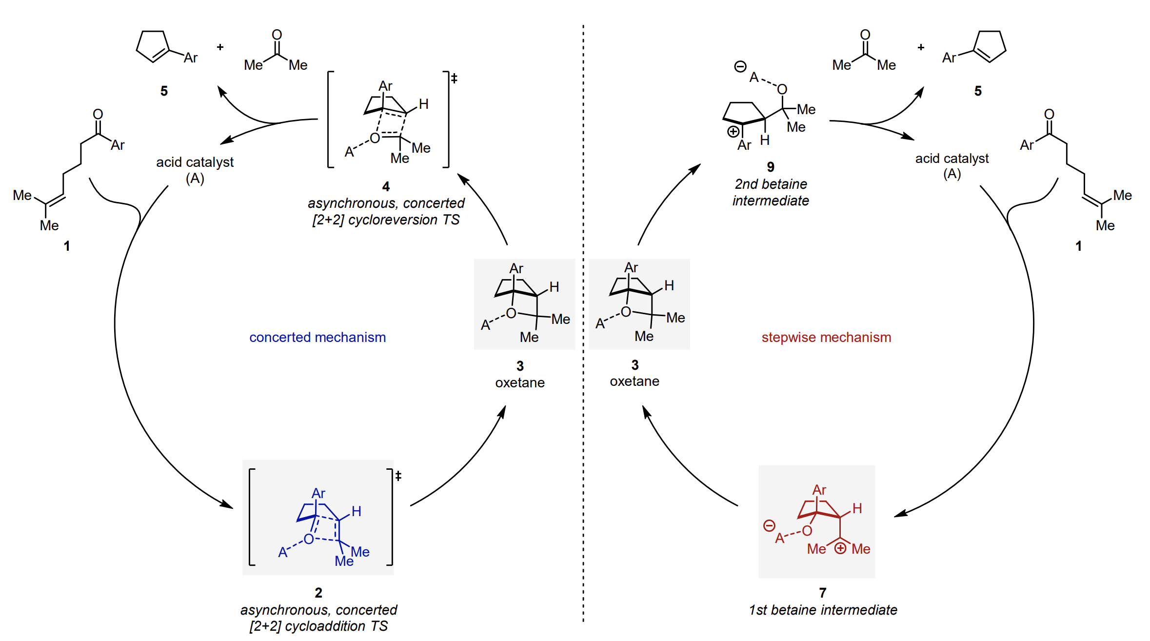
Detail of Figure 1 from Vonesh et al.
We approached this challenge with a battery of experimental and computational techniques. Careful natural-abundance 12C/13C KIE experiments conducted by Hannah, Eugene, and Spencer provided evidence for a stepwise mechanism, and Hammett studies supported this hypothesis—all experimental data we acquired were consistent with a stepwise mechanism, leaving only the computations to support a concerted 2+2 cycloaddition.
We hypothesized that the standard implicit-solvent models we were using were systematically understabilizing the betaine intermediate, leading to an erroneous prediction of a concerted mechanism. To test this assumption, Eugene and I ran ab initio molecular dynamics simulations to probe if explicit solvent and free-energy calculations could bring the computation into closer agreement with the experiment. These calculations were fantastically expensive: even using the smallest model system possible and trimming the functionals and basis sets to the absolute limit, each 1 fs timestep took 4–5 minutes of CPU time to complete, for an overall simulation throughput of around 0.4 ps per day.
After months of work, we were able to run umbrella sampling with 130 different 20-ps trajectories and use the 2D weighted-histogram analysis method to build a combined free-energy surface. Our results confirmed our hypothesis: the explicit-solvent free-energy surface has a clear minimum for the betaine intermediate, suggesting that the previously predicted concerted mechanism arises from failures in the implicit solvent model.
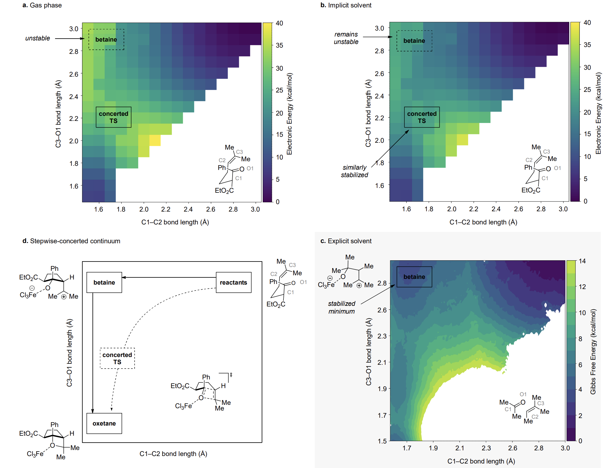
Detail of Figure 7 from Vonesh et al.
While this was an exciting result for the team, the extreme computational effort and expense required meant that it couldn't become a routine part of the computational toolkit.
Today, things are different: neural network potentials allow for high-quality simulations to be run many orders of magnitude faster than DFT, and improvements in coding agents dramatically reduce the effort and time associated with managing and deploying batches of trajectories. On our most recent Rowan company retreat, I decided to try modeling the COM reaction mechanism again with a modern computational stack.
Methodology
In the 2022 Vonesh work, we had to take a lot of shortcuts to make the simulation possible. We used a truncated reactive system (see above) inside a non-periodic cluster of 100 DCE molecules, with loose restraints keeping the solute in the center of the cluster. For forces, we used two-layer mechanical embedding: B3LYP-D3(BJ)/MIDI!/LANL2DZ(Fe,Cl) was used for the reactive solute system, while GFN0-xTB was used for the solvent. (This somewhat contrived combination of basis sets was found by benchmarking against DLPNO-CCSD(T) data; we made the basis set smaller and smaller until we couldn't squeeze out any more performance.)
For this new study, we were able to use a single NNP to cover the entire system. We studied the full substrate with 128 DCE molecules (1,070 total atoms) in an orthorhombic periodic box. Initial configurations were generated with Packmol, and c. 1 ns NPT MD was run to equilibrate the solvent configurations; OPLS-AA was used for DCE, while GFN2-xTB charges and UFF vdW parameters were used for the (frozen) solute.
Production simulations used OrbMol-v1-direct to compute forces. UMA-S-1.2 (with fast-inference mode), OrbMol-v2, and OrbMol-v1-conservative were also investigated but found to be meaningfully slower. This has implications: OrbMol-v1 doesn't explicitly handle long-range electrostatics, which may or may not be an issue (see my blog post on long-range forces in NNPs), and direct prediction of forces can lead to certain pathologies in optimization (although these probably aren't relevant when running NVT molecular dynamics).
With batch inference, OrbMol-v1-direct achieved amortized per-replica inference latency of about 37 ms per timestep on an NVIDIA A100 GPU. This is over 100x faster than the DFT calculations in the 2022 study, despite the fact that we were modeling approximately 37x more atoms (29 atoms with DFT vs 1070 atoms with OrbMol). We used a similar umbrella-sampling scheme to the 2022 study, running 82 100-ps simulations for a total of 8.02 ns of simulation (three simulations didn't quite finish). For comparison, the 2022 study ran 130 20-ps simulations for a total of 2.6 ns.
The entire project was completed in about two days, start to finish, with heavy use of coding agents. All simulations were run on Modal for a total of $262, including various experiments that didn't make it into the final study. Implementation was done with GPT-6.1 Sol and primarily used ASE and PyMBAR, with ancillary PyTorch and OpenMM code to boot.
Results
At a high level, the results agree with the 2022 study. There's a clear minimum in the betaine region, indicating that the reaction proceeds through a stepwise mechanism and not, as previous DFT calculations predicted, a concerted 2+2 cycloaddition.
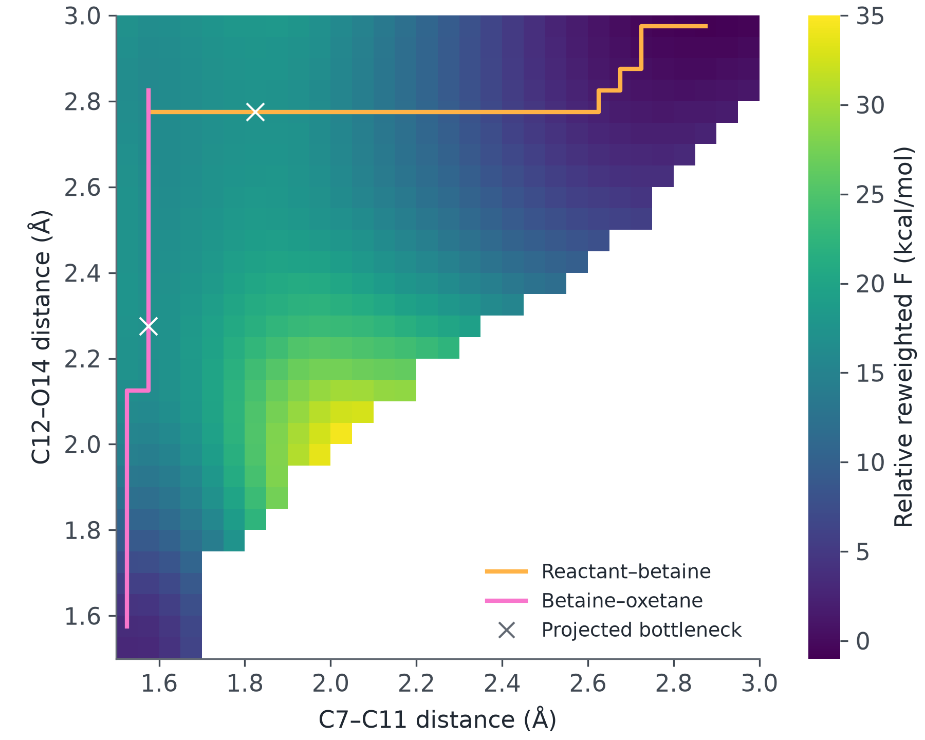
More O'Ferrall–Jencks plots, with predicted bottlenecks and paths overlaid
Looking at the free-energy surface, we can estimate the energies of the reactant–betaine TS (17.46 kcal/mol), the shallow betaine intermediate (16.01 kcal/mol), and the betaine–oxetane bottleneck (17.05 kcal/mol). Even with 100 ps per window, which is 5x longer than the previous study, there's meaningful disagreement between first-half and second-half free-energy estimates. Longer simulations would be necessary for fully converged results, although the trend is clear.
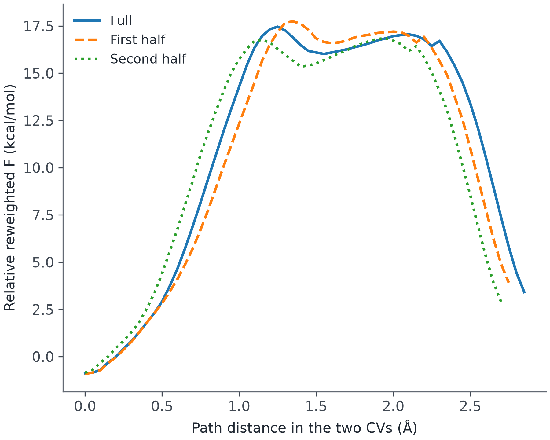
Free-energy surface generated in this study
Solvent Effects
The failure of the implicit-solvent model implies that the solvent is interacting with the betaine in an interesting way. We studied this in a few different ways.
First, we followed Singleton in looking at the solvent's electrostatic stabilization of the solute along the potential-energy surface. Using fixed OPLS charges, we investigated how strongly the solvent electrostatic configuration (within a 10 Å radius) interacted with a model C–O charge-pair probe. While the solvent electrostatics led to moderate stabilization in the reactant region (–1.0 kcal/mol) and the oxetane region (–4.9 kcal/mol), the betaine region saw stabilization of –16.6 kcal/mol. While this is not a solvation free energy, it suggests that solvent reorganization plays a significant role in stabilizing the developing carbocation.
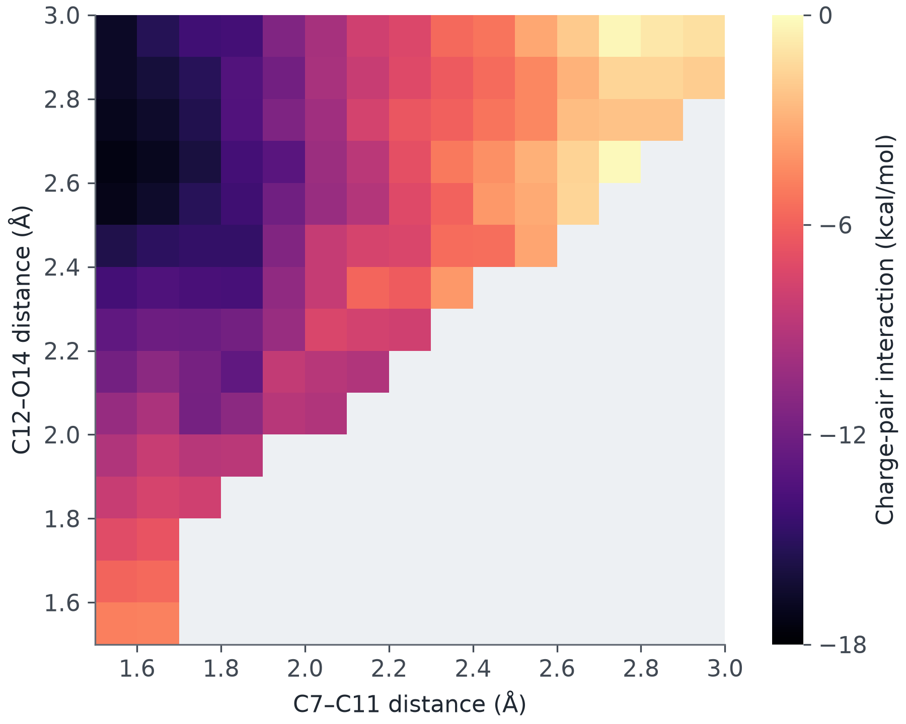
Solvent electrostatic interaction with charge-pair probe
We also probed specific solvent–solute interactions. The betaine region had markedly more contacts between DCE chlorines and the formally cationic carbon atom (C12) of the betaine (3.6x more than background), and nearby solvent dipoles reorient to better stabilize the cation. Solvent–C12 contacts were also more persistent in the betaine region: 23–31% of initial contacts survived for at least 1 ps in selected betaine windows, compared with 5–16% in reactant windows. It's worth noting that the presence of explicit chlorine–solute interactions is consistent with the reaction's observed preference for chlorinated solvents.
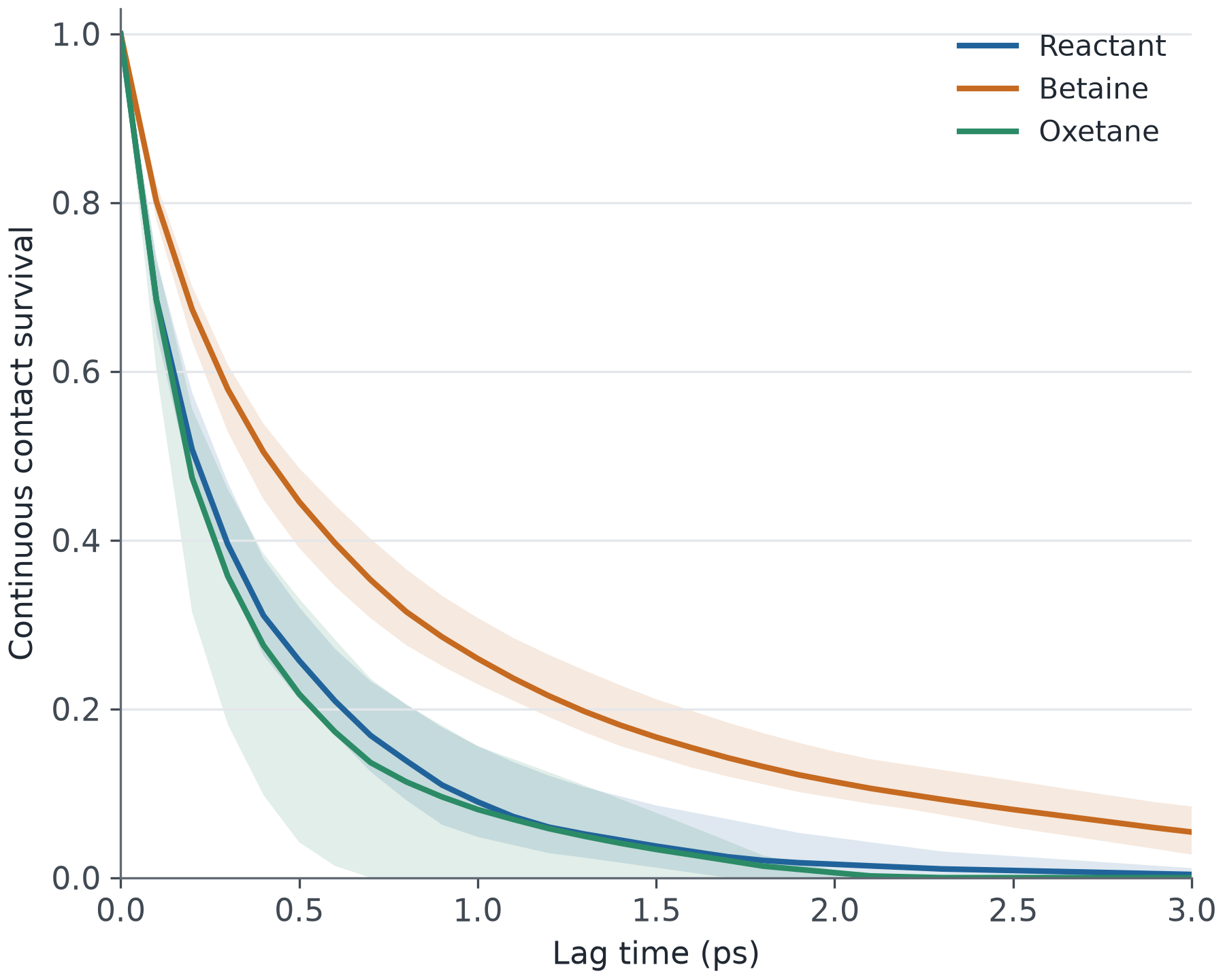
Solvent-contact survival plot
Trajectories
We initialized 16 trajectories from the saddle points and studied their evolution forwards and backwards in time. Of the 16 trajectory pairs, 3 successfully connected the reactant and oxetane wells. 2 of these trajectories passed quickly through the betaine region (total betaine residence times of 30 and 47 fs), while the last trajectory lingered (total betaine residence time of 485 fs).
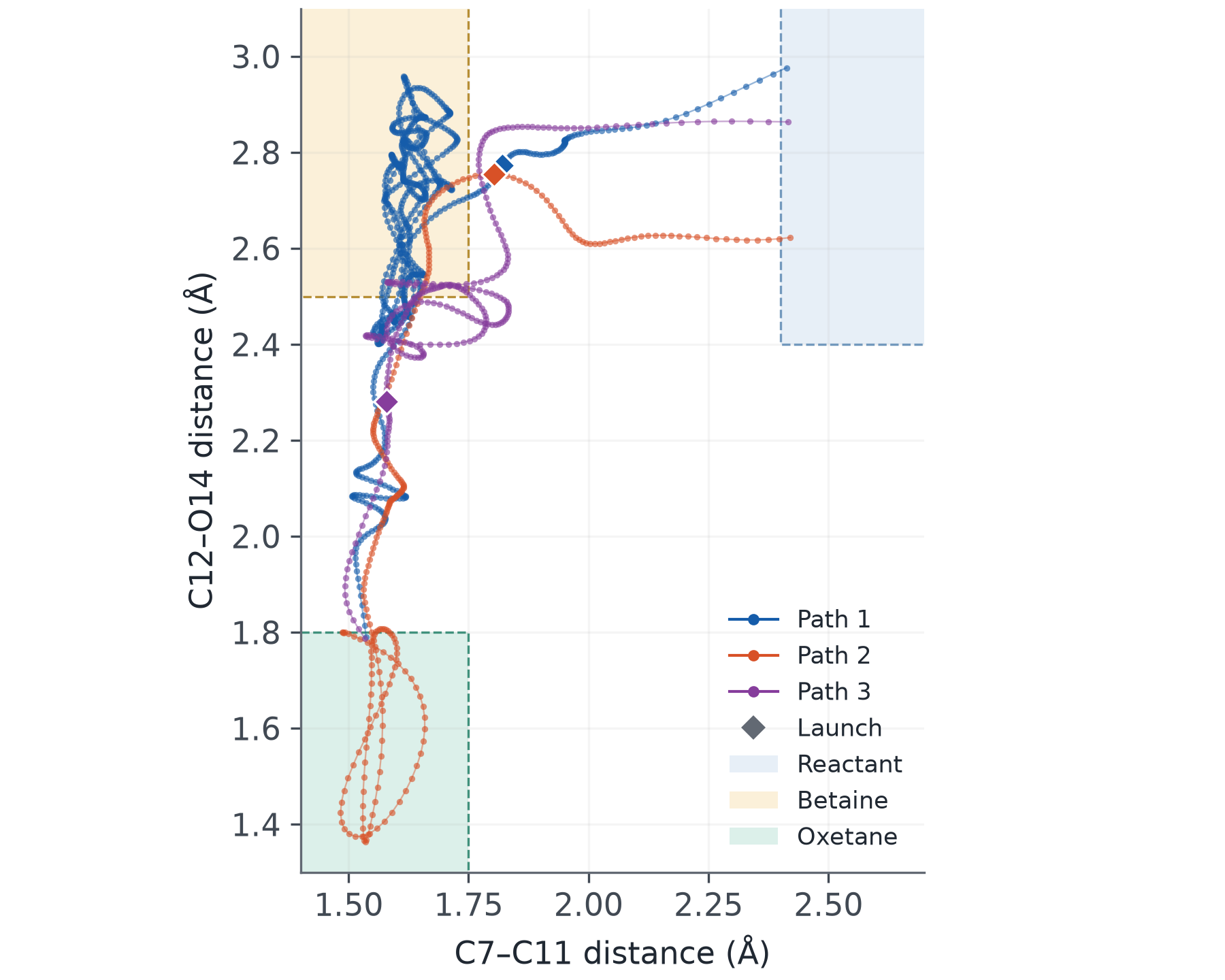
The three trajectories connecting reactant and oxetane wells
These studies give preliminary evidence for the potential importance of non-equilibrium solvation in this system. Reactants might pass through the betaine region faster than the solvent can reorganize to stabilize developing charge, leading to shorter intermediate lifetimes than a static free-energy analysis would predict. But these results are tentative and much more analysis would be needed to pin this down; see inter alia Roytman and Singleton's study of diene hydrochlorination for what this might look like (a study which was very influential on me as a mechanistic organic chemist).
Conclusions
Zooming out, the results from this NNP-powered simulation match the results Eugene and I obtained five years ago. This reproduction gives me additional confidence that our previous conclusion was correct and not an artifact of the specific design choices we employed—it seems very likely that Fe-catalyzed COM proceeds through a stepwise mechanism and not, as was previously proposed, a concerted 2+2 cycloaddition. The exact nature of the intermediate (dynamic intermediate? entropic intermediate?) I leave as an open question to future physical organic chemists; I'm out of the game, as they say.
This project was much easier the second time around. With modern NNPs and coding agents, simulations that used to take months of painstaking scientific work and high-performance computing can now be run overnight without having to manually write any code at all. As a fan of ab initio molecular dynamics, I hope that we'll see many more papers using these techniques to investigate reactions of interest to "ordinary" organic chemists; see my recent perspective with Dean Tantillo, Steven Lopez, and Eric Jacobsen!
Running these simulations also drove home how much the field still needs faster NNPs. OrbMol is many orders of magnitude faster than DFT, but an NNP that could run 10–100x faster would make it possible to run significantly more sampling and trajectories. I have no doubt that such speedups are coming (e.g. Vitrify), and the field of reactivity modeling will see immediate benefits from such speedups. We're approaching an era in which mesoscale phenomena can be modeled as routinely as nanoscale phenomena have been modeled, and this will change how most fields of chemistry operate.