Testing Binding-Affinity Prediction in Rowan
by Zachary Fried · Oct 13, 2026
We recently introduced Rowan's binding-affinity workflow, which provides several ways to score protein–ligand binding. These include three ML models: GNINA and AEV-PLIG, which use trained neural networks to estimate binding affinity from the supplied protein–ligand structure, and Nesso-1, which predicts affinity from protein sequence and ligand SMILES without requiring a pose.
You can also calculate binding affinity from single-point interaction energies. This approach first evaluates the energy of a ligand and the surrounding protein residues together, then subtracts the energies of the separated fragments:
The default calculation uses PM6-D3H4X with COSMO2 implicit solvation, drawing on the interaction-energy component of SQM2.20. It is important to note that our implementation omits the separate ligand conformational, proton-transfer, and entropy terms from SQM2.20, so the result is an interaction-energy score rather than a full estimate of binding free energy.
While we've defaulted to SQM2.20-style PM6-D3H4X/COSMO2 energies, you can choose any of Rowan's supported levels of theory, including neural network potentials and semiempirical methods, and customize the solvation and pose-optimization settings. Around the time we released the binding-affinity workflow, SandboxAQ introduced taqo, which uses the same energy-difference formulation with neural network potentials. Their results suggested that these relatively simple calculations could give useful rankings within a series of related compounds.
We therefore tested several methods in Rowan on the eight targets from the JACS benchmark (Wang et al. 2015) included in the taqo study: BACE, CDK2, JNK1, MCL1, p38, PTP1B, thrombin, and TYK2. Across these systems, we evaluated 199 ligand records to see how the methods performed and how much the results depended on structure optimization and the selected protein region.
How we ran the tests
We started from the supplied benchmark poses, retained the supplied protonation states, and removed waters.
For our calculations, we used a 6 Å truncation radius for every target except thrombin, where convergence problems in the initial g-xTB runs led us to use a smaller 4 Å pocket across all methods for consistency. The workflow automatically selects protein atoms within this distance of any input ligand, expands the selection to whole residues, and caps the cut bonds with hydrogens. It uses this same set of protein residues to calculate an interaction energy for each ligand individually.
We tested five energy methods: PM6-D3H4X, g-xTB, AIMNet2-ωB97M-D3, UMA-S-1.2, and OMol25-eSEN-sm-cons (henceforth abbreviated to "eSEN-sm-cons"). PM6 used the COSMO2 implicit-solvent model during single-point scoring, while the other four ran without solvation. (This might seem a bit odd but follows the taqo precedent.)
We compared two approaches. First, we calculated interaction energies directly on the supplied poses without optimization (SP). Second, we used the binding-affinity workflow's built-in optimization, which relaxes only the ligand while keeping the protein and caps fixed, followed by single-point scoring (opt→SP). This differs from taqo's structure preparation, which used molecular-mechanics minimization with implicit solvent before scoring and allowed nearby protein residues to relax under positional restraints.
The benchmark dataset includes experimental binding affinities, which we used to evaluate how well each method ranked the compounds within each target.
Interaction-energy results
The following table shows the opt→SP results alongside taqo's published UMA-S-1.2 and eSEN-sm-cons results. Taqo used eSEN-sm-cons for its headline comparisons with RBFE. All ranking correlations in the tables are Kendall's τ-b, with higher values indicating better agreement with the experimental rankings. As can be seen, performance varies quite a bit by target and energy method.
| Target | PM6-D3H4X | g-xTB | AIMNet2 | Rowan UMA-S-1.2 | taqo UMA-S-1.2 | Rowan eSEN-sm-cons | taqo eSEN-sm-cons |
|---|---|---|---|---|---|---|---|
| CDK2 | 0.31 (13/16) | 0.45 (15/16) | 0.40 | 0.45 | 0.62 | 0.43 (15/16) | 0.62 |
| JNK1 | 0.12 (00/00) | 0.52 (00/00) | 0.36 | 0.49 | 0.44 | 0.46 (00/00) | 0.42 |
| MCL1 | 0.49 (40/42) | 0.45 (40/42) | 0.10 | 0.53 | 0.62 | 0.56 (00/00) | 0.58 |
| p38 | −0.04 (00/00) | 0.37 (00/00) | 0.11 | 0.44 | 0.48 | 0.44 (00/00) | 0.48 |
| PTP1B | 0.27 (00/00) | 0.60 (00/00) | 0.52 | 0.57 | 0.61 | 0.60 (00/00) | 0.63 |
| Thrombin | 0.56 (00/00) | 0.64 (00/00) | 0.05 | 0.53 | 0.45 | 0.53 (00/00) | 0.56 |
| TYK2 | 0.57 (00/00) | 0.50 (00/00) | 0.33 | 0.50 | 0.48 | 0.48 (00/00) | 0.48 |
| BACE | −0.09 (34/36) | 0.06 (00/00) | 0.17 | −0.01 | 0.40 | 0.41 (00/00) | 0.46 |
| Mean | 0.27 (00/00) | 0.45 (00/00) | 0.26 | 0.44 | 0.51 | 0.49 (00/00) | 0.53 |
| Median | 0.29 (00/00) | 0.48 (00/00) | 0.25 | 0.50 | 0.48 | 0.47 (00/00) | 0.52 |
| Mean time (min/ligand) | 5.40 (00/00) | 3.59 (00/00) | 0.25 | 0.26 | — | 0.36 (00/00) | — |
Table 1. Kendall's τ-b for opt→SP interaction energies in Rowan alongside taqo's published values. Counts in parentheses show how many ligands were successfully scored out of the total; the remaining calculations failed or did not converge. Average runtimes include all submitted ligands, including failed and unconverged attempts, except for one unconverged g-xTB calculation for an MCL1 ligand that was a substantial runtime outlier.
The eSEN results show encouraging agreement with taqo despite the differences in structure preparation and pocket selection. Correlations are within 0.05 of taqo's reported values for seven of the eight targets, with a mean of 0.49 compared with 0.53. CDK2 shows the largest gap, although our result also excludes one ligand.
eSEN gives the highest mean correlation among the energy methods we tested. It also performs fairly consistently across targets, including BACE, where its correlation of 0.41 is close to taqo's 0.46. This contrasts with UMA's −0.01 on BACE and shows how much the choice of energy model can matter.
UMA also shows broadly similar correlations to taqo on most targets, with BACE being the main exception (which we'll return to below). For both UMA and eSEN, taqo's mean correlations are somewhat higher than ours. The additional protein relaxation in taqo's workflow may contribute to this, but differences in pocket selection could also play a role.
The following plot compares ligand-ranking performance across the eight targets for Rowan eSEN, taqo eSEN, g-xTB, AEV-PLIG, and Nesso-1. The Rowan eSEN and g-xTB results use opt→SP, while Nesso-1 uses protein sequences and ligand SMILES, and AEV-PLIG uses the original, unoptimized protein–ligand structures. We discuss the ML scoring methods in more detail below.
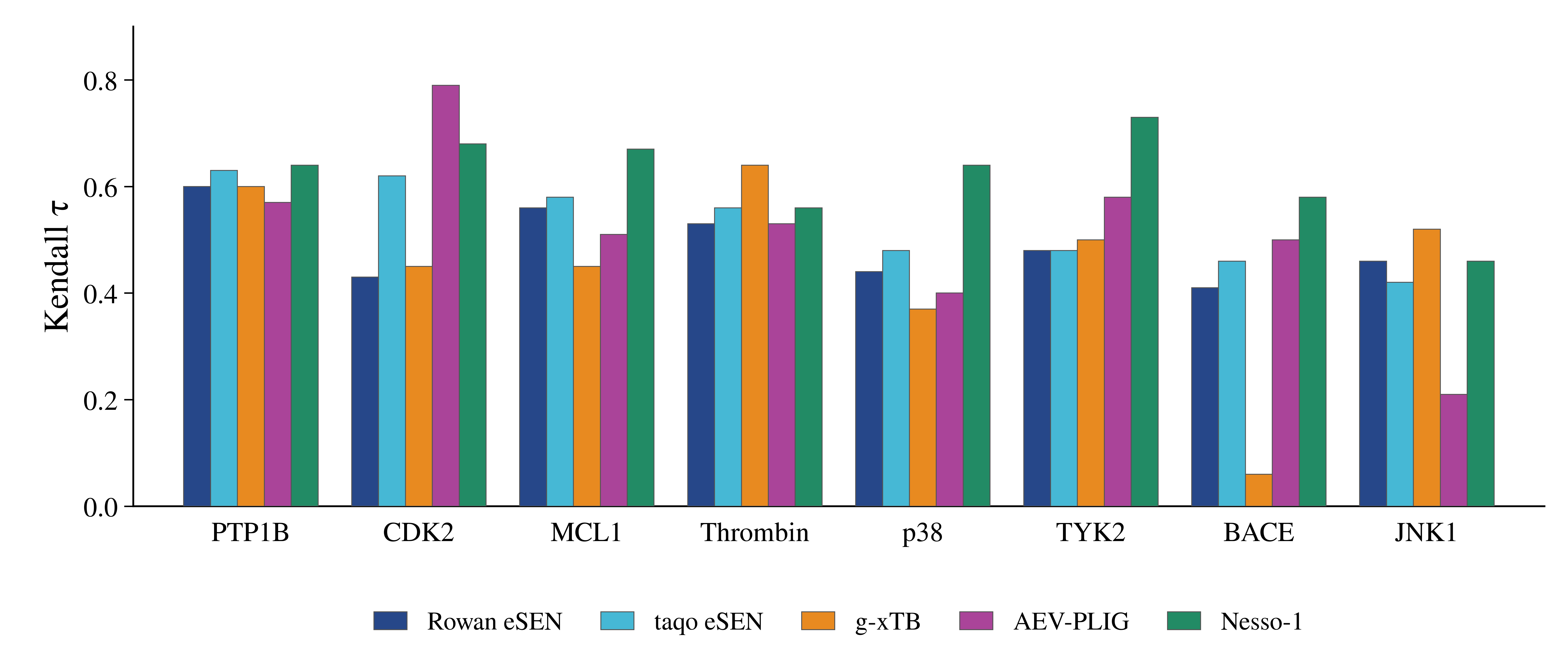
Figure 1. Ligand-ranking performance (Kendall's τ-b) across the eight JACS targets. Rowan eSEN and g-xTB use opt→SP interaction energies, AEV-PLIG scores the original poses, and Nesso-1 uses protein sequence and ligand SMILES.
Overall, there isn't one energy method that works best everywhere. Having these options in the same workflow makes it straightforward to test which settings work for a particular series. The differences also raise two practical questions: how much does relaxing the starting pose help, and how much does the selected protein region matter?
How much does optimization matter?
To look more closely at the starting geometry, we compared eSEN scores calculated directly on the original poses with scores after protein-aware ligand optimization. Single-point scoring without optimization was about 2.3–8.7× faster than opt→SP, depending on the energy method.
| Target | eSEN SP | eSEN opt→SP |
|---|---|---|
| CDK2 | −0.27 | 0.43 (15/16) |
| JNK1 | 0.42 | 0.46 (00/00) |
| MCL1 | 0.16 | 0.56 (00/00) |
| p38 | 0.47 | 0.44 (00/00) |
| PTP1B | 0.61 | 0.60 (00/00) |
| Thrombin | 0.49 | 0.53 (00/00) |
| TYK2 | 0.45 | 0.48 (00/00) |
| BACE | −0.12 | 0.41 (00/00) |
Table 2. Kendall's τ-b for eSEN-sm-cons interaction energies computed on the original poses (SP) and after ligand optimization (opt→SP).
The biggest improvements occur for CDK2, BACE, and MCL1. For CDK2, ligand optimization changes the correlation from −0.27 to 0.43. For BACE, it improves from −0.12 to 0.41, and for MCL1, from 0.16 to 0.56.
Both CDK2 and MCL1 contain severe clashes in their original, unoptimized structures: 8 of 16 CDK2 ligands and 7 of 42 MCL1 ligands had at least one severe ligand–receptor clash (defined as a pair of heavy atoms whose separation is more than 1 Å shorter than the sum of their van der Waals radii). This was previously observed by Pecina and co-workers. These contacts can produce large repulsive energies that obscure the differences we want to compare. The improvements after optimization suggest that cleaning up severe clashes is an important step before using single-point interaction energies to rank compounds.
Optimization didn't improve the rankings for every system, but it made a notable difference for CDK2, BACE, and MCL1. The practical takeaway is that an optimization step is especially important when the starting poses contain severe clashes. While these clashes are immaterial to RBFE calculations that will run nanoseconds of MD based on the starting poses, they're very bad for physics-based single-point methods!
BACE and the importance of residue selection
BACE gives poor rankings across most of the energy methods we tested, with eSEN being the exception. The UMA discrepancy is particularly large: our opt→SP correlation is −0.01, compared with taqo's reported value of 0.40. This led us to look more closely at the selected protein region.
Upon closer inspection, we realized that the taqo authors treated BACE differently than the other systems. Taqo typically selects residues using a 12 Å cutoff from a reference ligand's centroid, but the authors reduced this to 8 Å for BACE to leave out more distant charged residues. That choice changes the environment used to calculate the interaction energy. In particular, including or excluding charged residues alters the net charge of the protein system, which can shift the interaction energies and affect the ranking.
We also tested different truncation radii for BACE using UMA. Reducing the radius from 6 Å to 4 Å improved UMA's opt→SP correlation from −0.01 to 0.14, while a 2 Å cutoff gave a Kendall's τ-b value of 0.21. It's important to note that taqo selects residues based on their distance from a single reference ligand's centroid, while our workflow selects residues within the cutoff of any atom of any ligand in the batch. A 6 Å cutoff therefore defines different protein regions in the two workflows.
The smaller regions helped, although the UMA rankings remained poor. This sensitivity highlights the importance of controlling which residues enter the calculation. Using Rowan's workflow, you can define the protein region either by adjusting the truncation radius, as we tested here, or by supplying a specific set of residues to include.
How do the ML affinity models compare?
We also evaluated GNINA, AEV-PLIG, and Nesso-1 on the same benchmark. GNINA and AEV-PLIG scored the original poses without additional optimization, while Nesso-1 used sequence and SMILES. Here's how they compare with eSEN opt→SP:
| Target | GNINA | AEV-PLIG | Nesso-1 | eSEN opt→SP |
|---|---|---|---|---|
| CDK2 | 0.40 | 0.79 | 0.68 | 0.43 (15/16) |
| JNK1 | 0.37 | 0.21 | 0.46 | 0.46 (00/00) |
| MCL1 | 0.35 | 0.51 | 0.67 | 0.56 (00/00) |
| p38 | 0.52 | 0.40 | 0.64 | 0.44 (00/00) |
| PTP1B | 0.64 | 0.57 | 0.64 | 0.60 (00/00) |
| Thrombin | 0.71 | 0.53 | 0.56 | 0.53 (00/00) |
| TYK2 | 0.00 | 0.58 | 0.73 | 0.48 (00/00) |
| BACE | −0.04 | 0.50 | 0.58 | 0.41 (00/00) |
| Mean | 0.37 | 0.51 | 0.62 | 0.49 (00/00) |
| Median | 0.38 | 0.52 | 0.64 | 0.47 (00/00) |
| Mean time (min/ligand) | 0.12 | 0.02 | 0.10 | 0.36 (00/00) |
Table 3. Kendall's τ-b for the ML affinity models compared with eSEN-sm-cons opt→SP interaction energies.
Potential overlap with training data makes ML benchmarks harder to interpret. Both AEV-PLIG and Nesso-1 have published training protocols with exclusions that appear to cover these JACS sets: AEV-PLIG filters out similar training ligands using a fingerprint Tanimoto cutoff of 0.9, while Nesso-1 excludes examples with at least 90% protein sequence similarity to a benchmark target when training its binding-affinity head. These filters reduce overlap, but related chemistry can still remain in the affinity-training data. With this caveat in mind, the results, especially for AEV-PLIG and Nesso-1, are encouraging.
Brief final thoughts
The taqo results suggest that NNP single-point interaction energies are useful for ranking close analogues that share a binding mode, where omitted solvation and entropy contributions may largely cancel. In our own experiments on hit-classification datasets like DUDE-Z, these scores were less effective at separating hits from decoys, possibly because those contributions vary more across chemically diverse compounds.
If you're interested in running single-point binding-affinity calculations, or any of the other calculations discussed in this post, consider using Rowan!